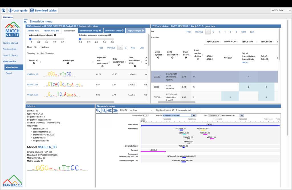
Predicting TFBS from geneXplain platform interface
TFBS prediction from single sequences to whole genomes (in the geneXplain platform via GUI or API)
In the geneXplain platform interface you will find a great variety of methods and workflows for TFBS prediction. The tools include standard site search with TRANSFAC database, sequence enrichment analysis, as well as AI-driven combinatorial analysis of TFBS provided by the Composite Module Analyst algorithm and Combinatorial models based on sparse logistic regression (MEALR).
Page Navigation:
Search for TF binding sites with TRANSFAC®
Analyze any DNA sequence for site enrichment with TRANSFAC®
Combinatorial analysis (AI and ML)
Construction of composite modules
Hierarchical structure of the composite modules
Construct composite modules results visualization and interpretation
Score calculation of the composite models
Combinatorial models based on sparse logistic regression (MEALR)
Combinatorial regulation analysis of genomic or custom sequences
MEALR combinatorial regulation analysis
Extract TRANSFAC® PWMs from combinatorial regulation analysis
Mapping TFBS on peaks calculated from ChIP-seq data
Site search in ChIP-seq peaks: Version 1.2 (Classical)
Site search in ChIP-seq peaks: Version 2.0 (Adjusted p-values)
Site search in ChIP-seq peaks: Version 3.0 (MATCH (TM))
Search for composite modules on ChIP-seq peaks with TRANSFAC®
Search for discriminative sites with TRANSFAC® (MEALR)
Videos with TFBS prediction in geneXplain platform
General info
The TFBS prediction tools are located in the Analyses –> Methods –> Site analysis section of the platform, as well as in the Analyses –> Workflows –> TRANSFAC section of the platform. Selected tools for sequence analysis can be found under the Sequence analysis button of the platform start page:
You can find information on the profile selection (collection of positional weight matrices – PWMs – transcription factor binding models that will be used for performing the site search) in this document or in tabular format here.
Search for TF binding sites with TRANSFAC®
The Search for TF binding sites with TRANSFAC® workflow in the geneXplain platform is designed to search for putative transcription factor binding sites, TFBS, in any input DNA sequence in EMBL, Fasta or Genbank formats. Using this workflow you can analyze DNA sequences of any species and of any genomic regions. In the analysis results of this workflow you will find a summary table and a track with found sites in the input sequences.
The summary table gives the site density per thousand bp for each matrix in the input sequence:
Each row summarizes the information for one site model (PWM – positional weight matrix).
For each row, the column Site density per 1000bp shows the number of matches normalized per 1000 bp length for the sequences in the input set.
The track of found sites can be visualised in genome browser:
In the field Sequence (chromosome) you can find a dropdown menu. This feature helps to easily switch between visualizations of the sequences in the input set. In this particular example the input sequence set comprises ten individual promoter sequences, and each individual promoter can be visualized in the genome browser.
The same track of found sites can be opened as a table for tabular visualisation:
Each row of such table corresponds to one resulting TFBS and includes sequence names, site positions (the columnsFromandTo), siteLengthandStrand,scorecalculated by the algorithm and a site model (TRANSFAC® matrix). This table can be exported as a track in several different formats including intervals, bed, wig and more. DNA sequences can be exported in multi-FASTA format.
Additional visualisation options are available for selected rows of the Summary table: the Report on selected matrices button at the top menu panel of the platform will visualize the found TFBS in the input sequences. In this example, all matrices with a site density <5 were selected. The visualization results are shown below:
There are ten rows corresponding to the individual sequences in the input set. The column Sites view schematically represents the sequence length with mapped TFBSs. Matches for different matrices are shown in different colors. You can select individual matches by mouse click and get additional information in the Info box.
Analyze any DNA sequence for site enrichment with TRANSFAC®
The Analyze any DNA sequence for site enrichment with TRANSFAC® workflow in the geneXplain platform is designed to search for enriched TFBS in any input DNA sequence as compared to a background DNA sequence. The central part of this workflow is performed by two individual methods: Site search on track and Site search result optimization, both can be found in Analyses –> Methods –> Site analysis.
With this workflow you can analyze sequences of any species and any genomic region.
The input Yes and No sequence sets can be in EMBL, FASTA or GenBank format.
The analysis results of this workflow include several tables and tracks.
The Summary table provides the overview of the TFBS enriched in the Yes set as compared to the No set:
Each row summarizes the information for one site model (PWM – positional weight matri).
For each row, the columns Yes density per 1000bp and No density per 1000bp show the number of matches normalized per 1000 bp length for the sequences in the input Yes set and input No set, respectively. The Column Yes-No ratio is the ratio of the first two columns. The higher the Yes-No ratio, the higher is the enrichment of matches for the respective matrix in the Yes set. The matrix cutoff values as they are calculated by the program at the optimization step are shown in the column Model cutoff, and the last column shows the p-value of the corresponding event.
TFBSs can be further visualized in the Yes sequences by selecting one or several rows of the Summary table and clicking on the Report on selected matrices button at the top menu panel of the platform.
In this example, all matrices having a Yes-No ratio>3 were selected. The visualization results are shown below:
There are four rows corresponding to the individual sequences in the input Yes set. The column Sites view schematically represents the sequence length with mapped TFBSs. Matches for different matrices are shown in different colors. You can select individual matches by mouse click and get additional information in the Info box.
The track of found sites represents TFBSs that are over-represented in the Yes sequences versus the No sequences. It can be viewed in the genome browser:
In the field Sequence (chromosome) you can find a drop down menu. This feature helps to easily switch visualization between the sequences in the input set. In this particular example the Yes sequence set comprises four individual promoter sequences, and each individual promoter can be visualized in the genome browser.
The track of found sites that are over-represented in the Yes sequences versus the No sequences can also be viewed as a table, scores of the putative TFBS are optimized by the algorithm:
Each row of this table corresponds to one resulting TFBS, and includes its position in the Yes sequences (the columns From and To), length and strand, as well as a score calculated by the algorithm and a site model (matrix). This table can be exported as a track, in several different formats including intervals, bed, wig and more. DNA sequences can be exported in multi-FASTA format.
In case of analysis Human, Mouse or Rat data, as well as since recent release the Arabidopsis, Zebrafish, Nematoda, Fruit fly, Baker’s yeast, and Fission yeast data, additional tables will be outputted by the workflow: Transcription factors Ensembl and Transcription factors Entrez. These tables aim at showing transcription factors linked to the identified site models (matrices). These are potential candidate regulators of genes in the input Yes set. They are supposed to regulate transcription of Yes-genes via the identified enriched TFBSs.
You will find a much more detailed description of the sequence analysis workflows in the geneXplain platform in the respective chapter of the user manual.
Site search on gene set
The Site search on gene set method of the geneXplain platform provides you with an ability to search for putative TFBS in a set of genes. As input for the analysis two gene sets should be provided: Yes (e.g. differentially expressed in an experiment, test set) and No (set of background genes, control set) as well as positional range relative to the TSS and a collection of predefined weight matrices with a particular threshold (profile). The analysis can be done for Human, Mouse, Rat, Arabidopsis, Nematoda, Zebrafish, Fruit fly, Baker’s yeast, and Fission yeast genes.
The Site search on gene set analysis results contain one Summary table and six tracks: yes promoters, no promoters, yes sites, no sites, yes sites optimized, and no sites optimized.
An example of the summary table is shown below:
Each row summarizes the information for one PWM. For each selected matrix, the columns Yes density per 1000bp and No density per 1000bp show the number of matches normalized per 1000 bp length for the sequences in the input Yes set and input No set, respectively. The Column Yes-No ratio is the ratio of the first two columns. Only matrices with a Yes-No ratio higher than 1 are included in the summary table. The higher the Yes-No ratio, the higher is the enrichment of matches for the respective matrix in the Yes set. The matrix cutoff values as they are calculated by the program at the optimization step are shown in the column Model cutoff, and the last column shows the p-value of the corresponding event.
The Yes promoters and No promoters tracks represent promoters of the input gene sets. These tracks can be opened as tables:
This table lists the positions of the promoter areas selected for the analysis on particular chromosomes, as shown in the columns From and To. The column Strand shows the strand on which each particular promoter is located. This track can be dragged and dropped on a particular chromosome opened in the genome browser to visualize the localizations of the promoters.
The track Yes sites optimized visualizes those putative sites that are over-represented in the promoters of the Yes set versus the No set as they are located in the promoters of the Yes set. Putative TFBS are shown as a track, scores of the putative sites are optimized by the algorithm.
This track is a list of all putative TFBS found in one analysis, it can be opened as a table. Each row presents details for each individual match for every PWM. The columns Sequence (chromosome) name, From, To, Length and Strand show, correspondingly, genomic location of the match including chromosome number, start and end positions, strand and length of the match. The column Type contains information about the type of the elements, in this case all matches are considered as “TF binding site”. Further columns keep information about PWM producing each match (column Property: matrix) as well as score for the whole matrix (column Property: score). The column Property: siteModel contains the identifier for the corresponding site model, which is the matrix together with a cutoff applied (and in the example shown is identical to the matrix identifier).
Yes (No) sites tracks are very similar in structure. The major difference is that these tracks include putative binding sites before the cutoff optimization, and thus they contain more sites.
Additional visualisation options of found TFBS are available for individual genes and individual matrices. Different rows of the summary table can be selected and visualized using the “report on selected matrices” button from the top menu panel of the platform: This action will open two new files: a table and a track. The constructed track has the same structure as described above for other track files. Each row of the constructed table corresponds to one individual gene:
The column ID presents the Ensembl ID for each gene, and the gene symbol is shown in the column Symbol. The column Sites view shows a schematic representation for each gene, where blue bars correspond to gene starts and coding regions, and TFBSs for different matrices are shown by arrows of different colors. The column Total count shows the number of TFBSs for all matrices together in the promoter of each particular gene. The next columns are named as matrices in the summary table and represent the number of TFBSs for each matrix in each particular gene.
On the picture above the table is sorted by the column Total count, and on the top we can see those genes that contain the highest total number of sites. This table can be sorted by different columns corresponding to individual matrices, and then on the top you will see those genes that contain the highest number of sites for the matrix in focus. The TFBS color schema in this table can be customized. This table can be exported in tab-separated format (txt) or comma-separated format (csv).
A much more detailed description of the Site search on gene set method can be found in the respective chapter of the geneXplain platform user guide.
Site search on track
The Site search on track method of the geneXplain platform provides you with an ability to search for putative TFBS in an input track. As input for the analysis the track for performing the site search should be provided (e.g. the track of promoter regions of studied genes), as well as the sequence source of the track and the collection of binding models (PWMs) that should be used for the TFBS search.
The result of this method is the track of found sites, which can be visualized as a table:
Each row of the table presents details for each individual match for every PWM. The columns Sequence (chromosome) name, From, To, Length and Strand show, correspondingly, genomic location of the match including chromosome number, start and end positions, strand and length of the match. The column Type contains information about the type of the elements, in this case all matches are considered as “TF binding site”. Further columns keep information about PWM producing each match (column Property: siteModel) as well as a score of the core (column Property:coreScore) and a score for the whole matrix (column Property: score). For details about these scores, please see Kel, Alexander E., et al. “MATCH: a tool for searching transcription factor binding sites in DNA sequences.” Nucleic acids research 31.13 (2003): 3576-3579, LINK.
Combinatorial analysis (AI and ML)
Composite modules
Composite modules are combinations of several TFBSs that are found together in a set of regulatory sequences. We search for such combinations of TF binding sites that are overrepresented in the regulatory sequences under study compared to a background set of sequences. The search for composite modules can be performed in the geneXplain platform using our in-house implementation of a genetic algorithm called Composite Module Analyst [Waleev, T., et al. “Composite Module Analyst: identification of transcription factor binding site combinations using genetic algorithm.” Nucleic acids research 34.suppl_2 (2006): W541-W545. Link].
As input for the genetic algorithm we take the output of a site search analysis. There are two individual analysis functions available in the geneXplain platform:
- Construct composite modules analysis – this method works on the promoter sequences specified relative to TSS in the set of genes. As input, it takes the results of the Site search on gene set analysis function.
- Construct composite modules on tracks – this method works with any DNA sequences specified by their absolute genomic positions, and is very often applied for the analysis of ChIP-seq fragments. As input, it takes the results of the Site search on track analysis function.
they are different with respect to the type of sequences where the search for composite modules is done, and correspondingly with respect to the format of the input data.
Both analysis functions can be found in the Analyses –> Methods –> Site analysis section of the geneXplain platform.
A brief overview of the site search methods (Site search on gene set and Site search on track) that serve as input for the composite modules construction analyses was provided above.
Construction of composite modules
The Construct composite modules method enables the identification of combinations of several TFBSs in the promoters of the genes under study (Yes-set). The resulting composite module differentiates the Yes-set from a background set (No-set). This analysis should be launched on the results of Site search on gene set analysis with the selected Yes-set, No-set and a specified profile of matrices.
The Construct composite modules on tracks method is designed for identifying combinations of several TFBS in DNA sequences specified by their genomic positions (tracks). An example of a track that is very often used is a set of the ChIP-seq data. The resulting composite module differentiates between a Yes-track and a background (No-track). This analysis should be launched on the results of Site search on track analysis with the selected Yes-set, No-set and a specified profile of matrices.
Details on how to launch these analyses can be found in the respective chapter of the geneXplain platform user guide.
Hierarchical structure of the composite modules
Prior to going into the composite modules analysis results visualisation, we first provide an overview of how the composite modules are visualized. Composite modules may have a complex hierarchical structure consisting of two levels: site models and modules. The highest hierarchical level contains several modules and corresponds to the promoter model.
The first level, site model, corresponds to the individual site model, often based on one PWM. Names of the site models are often the same as the matrix names (in case the site models are based on a library of matrices). The site models are taken from the profile that was used in the site search. In the resulting schemas the site models are shown by blue boxes, for instance:
Within these boxes, there are two values below the site model. The first value is the threshold value for the score of the respective site model, which is determined by the genetic algorithm during the optimization process (here it is equal to 0.81); in some cases this value is equal to 0.0, which means that the original threshold value given in the profile was found by the algorithm to be the optimal one. The second value, in this example N=2, is the maximum number of best found individual matches (sites) for this site model which are taken into account for calculating the score of the module.
The next level, module, may contain several site models, shown within the light brown boxes:
The module is characterized by its width, the average length of DNA window containing matches for the mentioned site models. In the example, the module width is 237 bp. In the resulting schemasmodulesare shown in green boxes, and they are numbered, e.g. Module 1, Module 2, ….
In the input form you can define the complexity of the promoter model to be constructed by specifying the number of units of each level: number of modules, number of site models, and also the minimum and maximum numbers of individual sites to be considered.
For example, in the visualisation below the number of modules was specified from 2 to 3, and correspondingly the resulting promoter model contains three modules: Module 1, Module 2, and Module 3. The number of site models was specified from 2 to 2, which means that the search was performed for pairs of individual site models. Respectively, in the resulting image you can see that each module contains two site models highlighted by blue circles:
Construct composite modules results visualization and interpretation
Below we provide the results visualisation of the Construct composite modules analysis obtained for the demo input data set. The input parameters of the method that were used for the analysis launch were as follows:
As a result, the method constructed two tables (Model visualization on Yes set and Model visualization on No set), two tracks (Yes track and No track), and one histogram.
In the Model visualization on Yes set table the the primary results of the analysis are presented: the identified composite modules are shown in the promoters of the Yes set:
Each row in this table corresponds to one gene of the Yes set, and for each gene the Ensembl ID and the gene symbol are shown in the two first columns. The column Model displays a symbolic map of the gene promoter taken for the analysis, in this case -500/+100 relative to the TSS. Arrows of different colors correspond to individual TFBSs, and a gradient in grey corresponds to the statistical density of the identifiedcompositemodules. The most intensive grey color corresponds to the center of a composite module. Each individual TFBS on this map is clickable, and upon a click information is displayed in the Info box (bottom left corner in the tool). As an example, one blue arrow is selected on the promoter of the top gene in the screenshot above, and for this selected TFBS the following details are shown in Info box:
The last column in the table, Score, shows a score calculated for each promoter depending on the number of modules, site models, sites, their scores and other statistical parameters. The higher the score for a promoter, the better the differentiation of this promoter from the promoters of the No set. The column Score is used for default sorting of the table, with the highest scores on top.
In addition to that, at the bottom part of the tool in the Model visualization on Yes set table you can also see the schematic representation of the hierarchical structure of the identified composite module, as well as a comprehensive set of its statistical characteristics:
The Yes track provides essential information about the regulation of individual promoters and is therefore important to be included in the visualization of individual promoters by the genome browser.
The schematic visualization can be comfortably extended to a more detailed visualization for each individual promoter:
For a selected promoter, you can see a more detailed map, including the names of the matrices and the numbers of individual modules, M1 through M4. Each element of this interactive map has a corresponding check box. Unchecked elements will not be displayed on the map. De-selection is applied simultaneously to both: the detailed view of one promoter, and the table with the schematic representation of all promoters.
The table Model visualization on No set shows a visualization of the identified composite modules in the promoters of the No set.
The structure of this table is the same as that of the Model visualization on Yes set table, described above.
The function of the No track is to provide a possibility for a detailed visualization of no promoters in a way similar to that of the Yes track.
The distribution of scores for individual promoters is shown as a Histogram, where the promoter score value is shown on X axis and the percentage of promoters (% sequences) having this score is shown on the Y axis:
This histogram can be further interpreted applying the statistical characteristics described above.
The center, a vertical grey line, corresponds to the average score value and is equal to 3.44 in this example. Promoters from the No set with a score above 3.44 are shown in the histogram as blue bars to the right of the center, and they are referred to as false positives. In this example, the false positive rate is 16.82 %.
Promoters from the Yes set with a score below 3.44 are shown in the histogram as red bars to the left of the center, and they are referred to as false negatives. In this example, the false negative rate is 23.42 %.
A visual analysis of the histogram suggests that the Yes promoters with a score above 4.5 are very well separated from the No promoters, which means that for this part of the promoters the composite model constructed is most suitable. In this example there are 38 promoters with the score value >4.5; they can be saved as a separate gene set, and for them the model obtained works best.
Score calculation of the composite models
The figure below demonstrates the calculation of the score value for the composite modules in the promoter sequences. The TSS is shown as a thin arrow on the right side of the figure. Four thick arrows exemplify four sites found in this promoter. The color of the arrows exemplifies the site model which these sites belong to (three site models – red, green and blue).
A promoter model consists of K modules. The score of each module Mk(Score(Mk),k= 1, …,K) is calculated according to this formula:
Here, Site Score (t,i) is the site score for the sites found in the promoter, which is calculated by the Match algorithm.
mt– the number of sites of the site model t found in the promoter.
Tk– the number of site models in the module Mk, and
The final promoter score is calculated as the sum of the module scores Mk.
Standard deviation (σ) of the normal distribution is subject of optimization by the genetic algorithm and represents the width of the module in the output of the composite module analysis.
Further details on the composite modules construction can be found in the respective chapter of the geneXplain platform user guide.
Combinatorial models based on sparse logistic regression (MEALR)
Combinatorial regulation analysis of genomic or custom sequences
This workflow scans input sequences for types of transcription factor binding regions represented in the library of MEALR models enclosed with TRANSFAC®. It is primarily intended to be applied for single sequence analysis.
The workflow proceeds through the following main steps.
- Prediction of potential binding locations using the TRANSFAC® MEALR combinatorial regulation analysis
- Extraction of TRANSFAC® PWMs represented by MEALR model hits using the Extract TRANSFAC® PWMs from combinatorial regulation analysis
- Preparation of a cutoff profile with extracted PWMs for subsequent MATCHTM search using the Create profile from site model table
- Prediction of binding sites represented by PWMs in input sequences using the TRANSFAC® MATCHTM for tracks
- The tools Filter track by condition and Intersect tracks are applied to derive filtered model predictions and intersections of predicted TF binding site and combinatorial model locations.
Prediction of functional transcription factor (TF) binding sites is a difficult task, because recognized DNA elements are rather short (typically between 10 and 20 base pairs) and often do not follow simple rules with regard to sequence specificity. Formation of TF-DNA complexes depends on a context determined by intertwining conditions like cellular differentiation, chromatin state, or expression and activity of cooperating TFs.
With almost 1000 human TFs, over 300 cell types and more than 50 tissue types, the TRANSFAC® library of MEALR models provides the first comprehensive collection of TF binding models that account for combinatorial TF-DNA complexes comprising multiple DNA-binding specificities as well as cellular and tissue-related contexts. These models can therefore deliver predictions with increased accuracy, so that subsequent searches for binding sites that mark the locations of individual TFs are able to focus on relevant PWMs. This is an important step to select from the large number of PWMs curated by TRANSFAC® and to prioritize binding sites of interest. Within longer sequences the MEALR model predictions furthermore suggest subregions where binding by certain TFs most likely occurs.
A much more detailed description of this workflow can be found here.
MEALR combinatorial regulation analysis
This analysis applies combinatorial regulatory models (CRMs) based on the MEALR affinity score [1] to classify or scan sequences for occurrences of combinations of transcription factor binding sites represented by TRANSFAC® PWMs. The models are taken from the MEALR library whose training data originate from the TRANSFAC® collection of high-throughput sequencing experiments.
The method can be launched either in a classification or in the scan mode. The Classification mode evaluates input sequences as a whole, whereas the scan mode analyzes sequence windows separated by the given step size (sliding window). In scan mode, the Best hit method reports the best scoring sequence window disregarding a cutoff and the Cutoff method reports the best non-overlapping windows satisfying the specified cutoff.
The output folder encompasses a table and sequence track with information about model hits. The output table contains sequence start and end points of hits, model ids, match probabilities as well as other values as described below. For input sequences derived from genomic regions (instead of imported as custom sequences) the table includes in addition a sequence id generated for a region as well as the genomic sequence id, start and end coordinates.
[1] Katie Lloyd, Stamatia Papoutsopoulou, Emily Smith, Philip Stegmaier, Francois Bergey, et al., The SysmedIBD Consortium; Using systems medicine to identify a therapeutic agent with potential for repurposing in inflammatory bowel disease. Dis Model Mech 1 November 2020; 13 (11): dmm044040.
A much more detailed description of this mathod can be found here.
Extract TRANSFAC® PWMs from combinatorial regulation analysis
This tool extracts TRANSFAC® PWMs from a result table generated by the MEALR combinatorial regulation analysis. The PWMs represent transcription factor binding specificities that constitute the combinatorial module predicted by the MEALR model.
The output contains the TRANSFAC® PWMs extracted from MEALR models according to specified cutoffs. This table can further be applied in several analyses, e.g. to extract corresponding transcription factors using the tool or to create a profile for binding site predictions ( Create profile from site model table) with MATCHTM.
A much more detailed description of this mathod can be found here.
Mapping TFBS on peaks calculated from ChIP-seq data
The geneXplain platform also provides tools for mapping of TFBS to the peaks calculated from ChIP-seq data. You will find respective workflows under the ChIP-seq button of the geneXplain platform main menu:
Site search in ChIP-seq peaks: Version 1.2 (Classical)
This workflow helps to map TFBS on peaks calculated from ChIP-seq data. Site search is done with the help of the TRANSFAC® library of positional weight matrices, PWMs, using the pre-computed profile vertebrate_non_redundant_minSUM.
The input track should be provided in the BED format and submitted to the analysis as the Yes track. The No track can be selected from the ready tracks of housekeeping genes or uploaded as a custom track of your choice.
The results of the workflow contain two tables: Site optimization summary and Transcription factors and two tracks: Yes sites opt and No sites opt.
The Site optimization summary table includes the matrices the hits of which are over-represented in the Yes track versus the No track. Only the matrices with Yes-No ratio higher than 1 are included in this output table. The hits of these matrices can be interpreted as over-represented in the Yes set versus No set:
Each row of this table summarizes the information for one PWM. For each selected matrix, the columns Yes density per 1000bp and No density per 1000bp show the number of matches normalized per 1000 bp length for the sequences in the input Yes set and input No set, respectively. The Column Yes-No ratio is the ratio of the first two columns. Only matrices with a Yes-No ratio higher than 1 are included in the summary table. The higher the Yes-No ratio, the higher is the enrichment of matches for the respective matrix in the Yes set. The matrix cutoff values as they are calculated by the program at the optimization step are shown in the column Model cutoff, and the last column shows the P-value of the corresponding event.
The Transcription factors table includes transcription factors (TFs) that are associated with the PWMs that are listed in the table Site optimization summary:
Each row of this table shows details for one TF, including its Ensembl gene ID (column ID), gene symbol, gene description and biological species of the corresponding TF (columns Gene description, Gene symbol, and Species). The column Site model ID shows the identifier of the PWM associated with this TF, and several further columns repeat information that is also shown in the table Site optimization summary.
Each row of the tracks Yes sites opt and No sites opt presents details for each individual match for every PWM:
Columns Sequence (chromosome) name, From, To, Length and Strand show the genomic location of the match including chromosome number, start and end positions, strand and length of the match, respectively. The column Type contains information about the type of the elements; in this case all matches are considered as “TF binding site”. Further columns keep information about PWM producing each match (column Property:matrix) as well as a score of the core (column Property:coreScore) and a score for the whole matrix (column Property:score). The column Property: siteModel contains an identifier for the site model, which is the matrix together with the cutoff applied (for details about these scores, please see Kel, Alexander E., et al. “MATCH: a tool for searching transcription factor binding sites in DNA sequences.” Nucleic acids research 31.13 (2003): 3576-3579, LINK.
The genome browser visualization of the constructed tracks is shown below:
Such a view may help to visually co-localize information on different tracks, e.g. putative TFBS with variations, repeats and genes. In the figure above, the cursor shows position 29444, and two variations are located at this position. You can immediately recognize that these variations are located within particular putative binding sites in the intron region of the WASH7P gene.
The same information is available not just as a picture, but also as a table. For each element information is shown on chromosome, positions, length, strand, type of the track, and name of the element:
This table can be exported as a track, in several different formats including intervals, bed, wig, gff, gtf and more.
The same workflow can be launched on multiple interval sets: in the input Yes tracks field several different tracks can be simultaneously submitted. The same background dataset, Input No track, is used for comparison with each of the submitted Yes tracks. The default No track corresponds to far upstream regions of the house keeping genes, where no functional TFBSs are expected. The workflow will iteratively perform the same steps for each of the input Yes tracks. This helps to save time and efforts, especially when you have several sets of ChIP-seq data, e.g. the peaks for a number of different TFs.
A much more detailed description of this workflow can be found here.
Site search in ChIP-seq peaks: Version 2.0 (Adjusted p-values)
This workflow is designed to map putative enriched TFBSs on peaks calculated from your ChIP-seq data (Yes set) as compared to a random background set (No set). Importantly, the No set is created automatically and contains by default 1000 intervals. In the first part of the workflow, the enriched motifs are identified by our proprietary MEALR approach.
Enriched motifs serve as a basis to construct a specific profile. At the next step this newly generated profile is run on the same list of input peaks applying the search for enriched TFBSs on tracks method.
The input track should be provided in the BED format as the Input Yes track – it is the track with peaks from your ChIP-seq study.
Select the profile (collection of PWMs to perform the search for TFBS) – vertebrate_non_redundant_minSUM by default (any other TRANSFAC® profile or custom user-specific profile can be selected).
A filter for the coefficient of the MEALR method should also be specified. The default filter is set as >0.125 to have 75% or more of true discovery rate, TDR. For 90% TDR, you can type 0.270 in this field and for 50% TDR – 0.05593. The filtered motifs are included in the output asenriched motifs. At the later step, PWMs corresponding to the enriched motifs are used to make a new profile.
In the results of the workflow you will find four tables (Enriched motifs MEALR, Transcription factors, Site search summary, Profile) and three tracks (Random No sites opt, Random No track and Yes sites opt filtered track), the folder with demo results of this workflow can be viewed here.
The table Enriched motifs MEALR includes enriched motifs in the Yes track versus the No track, filtered by the coefficient as specified.
Please note that by default only the matrices with a Coefficient > 0.125 (75%TrueDiscoveryRate) are included in this output table. These motifs can be interpreted as the best discriminating motifs between the Yes and No sets.
The table Enriched motifs MEALR shown below has been sorted by the values in the Coefficient column. The larger the coefficient, the more important the corresponding motif was for discriminating between Yes and No sequences:
The table Profile is opened automatically and is an input-specific profile, based on the filtered enriched motifs MEALR:
This profile is an intermediate result of the workflow and is used further for Site search on gene set analysis in the second part of the workflow.
The Transcription factors Ensembl table includes transcription factors (TFs) that are associated with the PWMs listed in the table Site search summary:
Each row of this table shows details for one TF, including its Ensembl gene ID (column ID), gene symbol, gene description and biological species of the corresponding TF (columns Gene description, Gene symbol, and Species). The column Site model ID shows the identifier of the PWM associated with this TF, and several further columns repeat information that is also shown in the table Site search summary.
A much more detailed description of this workflow can be found here.
Site search in ChIP-seq peaks: Version 3.0 (MATCH (TM))
This workflow is designed to search for enriched transcription factor binding sites (TFBSs) in a set of genomic sequences in comparison to a random background set. With this workflow you can analyze sequences from the genome of human, mouse, rat, arabidopsis or zebrafish. To identify enriched binding sites within the sequences, positional weight matrices from the TRANSFAC(R) database are used while performing the method TRANSFAC(R) MATCH(TM) for tracks. The site search result will be further converted into a table of potential transcription factors that can bind to the identified TFBSs. The identified enriched transcription factor binding sites can be visualized in the genome browser.
Genomic sequences in track format (input example) can be submitted for the input. A random track of 1000 sequences that does not overlap with the input sequences is automatically generated as the background set.
The results of the workflow contain several tables and tracks. The identified enriched transcription factor binding sites (TFBSs) are present in a summary table (result example) and can be visualized in the genome browser as a track (result example). The potential transcription factors are given in a final Ensembl table (result example) with annotated GeneSymbol IDs and a short description.
A much more detailed description of this workflow can be found here.
Search for composite modules on ChIP-seq peaks with TRANSFAC®
This workflow finds pairs of TFBSs that discriminate between two tracks, theYes and the No tracks. As the Yes track, the ChIP-seq peaks identified as binding profiles for particular transcription factors can be considered.
The ChIP-seq experimental technology is widely applied to a variety of biological problems, in particular to study genome-wide histone modification profiles, e.g. histone methylation and histone acetylation profiles. Correspondingly, the same workflow in the platform can be used to analyze histone modification profiles as well.
For an example let’s consider the results of the workflow application to find composite modules in the ChIP-seq peaks identified for in-vivo-bound fragments of transcription factor E2F1 in HeLa cells, published in Gene Expression Omnibus,GSM558469.
Input Yes track. The original track of genome-wide E2F1 binding fragments was filtered by the length shorter than 600 bp, which resulted in 249 fragments. This track of 249 fragments is used as the input Yes track. The track can be found here.
Input No track. A track of the far upstream fragments of the human housekeeping genes located on chromosome 1 is taken as the No track. The track can be found here.
The results of this analysis run can be found here.
The results contain the Site optimization summary table, which contains those site models that are over-represented in the Yes track as compared to the No track:
Each row of the table represents the result for one PWM from the input profile. Only those PWMs with Yes-No ratio >1 are included in the output. Upon sorting by the Yes-No ratio, matrices for E2F factors are among top 20 lines. Please note that the p-values of E2F matrices are extremely low, which demonstrates highest statistical significance of the results.
The Modules folder in the results of the workflow contains the found composite module. The composite module found on our example contains two pairs, and we can see by exactly which site models (matrices) these pairs are formed as well as the statistical parameters of the overall model. Both pairs contain matrices for E2F factors:
For further details on this workflow and its results interpretation please refer to the respective chapter of the geneXplain platform user guide.
Search for discriminative sites with TRANSFAC® (MEALR)
The tool MEALR finds combinations of TFBS matrices that discriminate between two sets of sequences (denoted asYes and No sets). TheYes set may consist of genomic regions identified in a ChIP-seq experiment. No sequences are often other non-coding genomic regions not overlapping with the peaks.
MEALR differs from other tools in the following points:
- No cutoff or threshold is used on matrix scores to determine potential binding sites. Instead, MEALR calculates threshold-free sequence scores.
- MEALR builds a discriminative model for classification which is well-established and widely applied in statistical analysis called Sparse Logistic Regression. The model consists of a linear model that estimates the probability that a sequence belongs to the Yes set based on its binding site features.
- The sparseness constraint enables MEALR to select a subset of matrices relevant for classification of Yes and No sequences from a possibly large matrix library. Therefore MEALR’s output differs from other tools by presenting a focused set of matrices.
- While other site enrichment tools provided in the platform evaluate enrichment separately for each matrix, the model used in MEALR assesses the importance of matrices for discrimination in combination with other matrices of the library. Therefore, MEALR suggests (linear) combinations of transcription factor motifs.
For each input sequence x MEALR calculates a score for each PWM by the following equation where W denotes the number
of windows scored by the PWM and LSmax(xw) is the high log-odds score of window w :
f(x) = log( Σw exp(LSmax(xw)) / W )
Each sequence is therefore associated with a vector of scores, one from each matrix, and a class (Yes, No).
Let us present an example analysis for a ChIP-seq data set consisting of 500 peak regions and 1000 sequences randomly sampled from regulatory regions across the human genome.
Yes set is the set of sequence intervals that you want to analyze, for example these can be ChIP-seq peak regions.
No set is the set of background intervals (control set).
In the input profile (collection of PWMs – binding motifs) the cutoffs will be ignored, because MEALR calculates whole sequence scores.
In the results of analysis the summary table would look like this:
A row of this table contains matrix identifier and its logistic regression coefficient. The larger the coefficient value, the more important the corresponding matrix was for discriminating between Yes and No sequences. In our example, three of the five top matrices represent members of the transcription factor subfamily C/EBP.
For further details on this method please refer to the respective chapter of the geneXplain platform user guide.