TRANSFAC 2.0

Discover
TF binding sites in promoters
and enhancers of your genes


  • PWMs over 10,000 for animals, plants, and fungi
  • MATCH the best site search and enrichment tool
  • TF Sites experimentally proven and ChIP-seq 
  • Promoters, Enhancers tissue and cell type-specific ( Hi-C, CAGE, single cell)  
  • Omics analysis RNA-seq, ChIP-seq, ATAC-seq, CUT&RUN, WGS, WES, single cell
  • AI and ML reveals site combinatorics 
  • Easy GUI for no-coding bioinformatics
  • Over 200 tools and pipelines Analyze genes, FASTA, FASTQ, VCF, BED.  
  • Cloud Storage 100GB
  • API run our tools from your local Python and R

Reconstruct
signal transduction network
controlling your genes


  • Master regulators Search upstream of TFs using modern graph algorithm
  • Upstream analysis promoter + network analysis 
  • Pathways signaling and metabolic
  • Reaction network over 1,200,000  experimentally proven reactions
  • SBGN viewer web pathway/network editable diagrams
  • ODE modeling the fastest and most robust simulation engine.

Identify
drug targets
and disease biomarkers


  • Disease mechanism discovery with AI and upstream analysis for over 3,900 human diseases
  • Biomarkers over 140,000 (causal, correlative, MOA) and over 2,000,000 annotations
  • Drugs and targets over 10,000 drugs and over 55,000 targets
  • Clinical trials over 1,100,000 trial-disease pairs
  • Drug repurposing using networks and chemoinformatics
  • Multi-omics integration “All Five”: transcriptomics, genomics, epigenomics, proteomics, metabolomics
  • Fully automatic one-click solution with graphical experiment design
  • Detailed report with everything needed for your paper

Discover
TF binding sites in promoters
and enhancers of your genes


  • PWMs over 10,000 for animals, plants, and fungi
  • MATCH the best site search and enrichment tool
  • TF Sites experimentally proven and ChIP-seq 
  • Promoters, Enhancers tissue and cell type-specific ( Hi-C, CAGE, single cell)  
  • Omics analysis RNA-seq, ChIP-seq, ATAC-seq, CUT&RUN, WGS, WES, single cell
  • AI and ML reveals site combinatorics 
  • Easy GUI for no-coding bioinformatics
  • Over 200 tools and pipelines Analyze genes, FASTA, FASTQ, VCF, BED.  
  • Cloud Storage 100GB
  • API run our tools from your local Python and R

Reconstruct
signal transduction network
controlling your genes  


  • Master regulators Search upstream of TFs using modern graph algorithm
  • Upstream analysis promoter + network analysis 
  • Pathways signaling and metabolic
  • Reaction network over 1,200,000  experimentally proven reactions
  • SBGN viewer web pathway/network editable diagrams
  • ODE modeling the fastest and most robust simulation engine.

Identify
drug targets
and disease biomarkers


  • Disease mechanism discovery with AI and upstream analysis for over 3,900 human diseases
  • Biomarkers over 140,000 (causal, correlative, MOA) and over 2,000,000 annotations
  • Drugs and targets over 10,000 drugs and over 55,000 targets
  • Clinical trials over 1,100,000 trial-disease pairs
  • Drug repurposing using networks and chemoinformatics
  • Multi-omics integration “All Five”: transcriptomics, genomics, epigenomics, proteomics, metabolomics
  • Fully automatic one-click solution with graphical experiment design
  • Detailed report with everything needed for your paper

TRANSFAC BASIC

Discover TF binding sites in promoters and enhancers of your genes

Introduction

TRANSFAC® is the database of eukaryotic transcription factors, their genomic binding sites and DNA-binding profiles. Dating back to a very early compilation 35 years ago, it has been carefully maintained and curated to become the gold standard in the field. Since then this biggest collection of transcription factors and their genomics binding sites has served the scientific community as the most reliable and comprehensive resource for gene regulation studies.

You can use TRANSFAC® as an encyclopedia of transcriptional regulation, or as a tool to identify potential TFBSs by applying its library of positional weight matrices, a unique collection of DNA-binding models. The latter can be done with the included MATCH (Suite) tools or with any of the respective modules in the geneXplain platform.

Database content

The core of TRANSFAC® comprises contents of two domains: One documents transcription factor-binding sites (TFBSs, SITES), usually in promoters or enhancers, and the derived DNA binding motifs in form of positional weight matrices (PWMs, MATRICES). The other describes the transcription factors (TFs, FACTORS) subsumed to classes, based on the general properties of their DNA-binding domains, which has been expanded to a comprehensive classification (TF CLASSIFICATION), the latest version of which can be found here.

TRANSFAC search interface

The TRANSFAC® database search interface is provided in the web browser online. 

PWMs:

Binding sites referring to the same TF are merged into a positional weight matrix. Such a matrix reflects the frequency with which each nucleotide is found in each position of this TF’s binding sites and, thus, the base preference in each position.

TRANSFAC® includes over 10,000 Positional Weight Matrices (PWMs) that are robust models for predicting TF binding sites in genomes of various animals, plants, and fungi.

TF Sites:

TRANSFAC® includes over 50,000 experimentally proven TF binding sites and about 100 million ChIP-seq TF binding regions.

TRANSFAC® site information include genomic coordinates of the site, transcription factors binding to the site and detailed experimental evidences of the TF binding and gene regulation by the site in the particular tissue and cellular conditions.

ChIP-seq sites

TRANSFAC® includes 100 million ChIP-seq TF binding regions.

TRANSFAC® ChIP-seq information is based on ENCODE project and on literature curation. All published peaks of the respective ChIP-seq experiments are incorporated TRANSFAC database and annotated by the proper links to the binding transcription factors. We also predicted the best binding sites in these peaks using TRANSFAC PWM library.

Promoters, Enhancers:

TRANSFAC® includes promoter genomic annotation for various vertebrate and invertebrate species as well as for plants and fungi. TRANSFAC® also includes genomic information for over 200,000 human enhancers and silences acting in different tissues and cell type-specific.

The enhancer and promoter data is accumulated from numerous public repositories of CAGE, FANTOM and Hi-C data in bulk and single cell.

Tools

Site Analysis

What is Site Analysis?

Binding sites for proteins in the genome have a great regulatory impact on the gene activities in their neighborhood. Since these interactions are highly dynamic with regard to the cell’s status, we have experimental knowledge about the actual occupancy of these sites only for a very small percentage of them. Predictive tools are thus essential for deciphering the full regulatory potential of gene control regions like promoters, enhancers, etc.

Approaches to site analysis

Among the most popular methods to identify potential transcription factor binding sites (TFBSs) is the use of position-specific scoring or positional weight matrices (PSSM or PWM). The TRANSFAC® database, the gold standard in the field, harbors the largest collection of PWMs. They are used to predict TFBSs either by MATCH Suite, which is part of the TRANSFAC®2.0 online resource, or by a number of programs that are included in the geneXplain platform.

Site analysis in the geneXplain platform

The sequence patterns individual TRANSFAC matrices represent and recognize are visualized as logo plots.

These matrices can be individually selected and combined to “profiles”; a number of pre-defined profiles are available for subsequent sequence analysis. Matrix matches are visualized along the gene sequences in a customizable manner.

Visualization of transcription factor binding sites (TFBSs) with geneXplain platform’s genome browser.
The built-in genome browser enables to comfortably zoom-out to chromosomal level, or to zoom-in to the nucleotide level. Individual sites are clickable to invoke detailed information.

Advanced promoter analysis

State-of-the-art analysis of regulatory regions has to exceed recognition of single sites. Functional promoters, and presumably enhancers and other regulatory regions, are characterized by specific arrays of individual sites. As variable as their compositions may be, the syntax of sites in each regulatory region has to follow defined rules, which are largely unknown yet.

Therefore, the geneXplain platform provides an empirical way to identify the specific combination of sites that characterizes a given set of co-regulating promoters.

Complex promoter analysis, visualization of transcription factor binding sites (TFBSs) constituting a “promoter model”. (Click Image for an enlarged view.)

These specific combinations, also called “promoter models”, can be further used for screening genomic sequences or promoter databases. A comprehensive collection of mammalian promoters comes along with the TRANSFAC® database in its TRANSPRO section. The density of model matches is visualized by graded shading.

Promoter analysis for matches with a model comprising a set of transcription factor binding sites (TFBSs). (Click Image for an enlarged view.)

Key features of the TRANSFAC BASIC package tools:

MATCH and FMatch:

TRANSFAC®  includes one of the best site search and site enrichment tools equipped with powerful user interfaces for application in different analysis tasks.

The TRANSFAC® database provides a wide variety of tools for predicting transcription factor binding sites (TFBS) in the studied DNA sequences. In the portal interface of the TRANSFAC® database you will find the Match, FMatch, and Composite Model analysis tools for TFBS prediction under the Tools menu button:

1. Match – search for TF binding sites

This option uses the Match algorithm, in combination with a selected profile containing a list of matrices and their assigned cut-offs to search for individual transcription factor binding sites that meet the specified cut-offs.The Match option is recommended when the broadest set of results is desired.

2. Composite model – search by pairs of TFs

This option uses the Composite Model algorithm, in combination with a selected model or models which represent pairs of transcription factors known to act together to coordinately control gene regulation, and their assigned cut-offs to search for pairs of transcription factor binding sites that meet the specified cut-offs.The Composite Model option is recommended when specific information about coordinate regulation is known, or when more stringent results are desired.

3. FMatch – search for overrepresented TF binding sites

This option is used to find sites which are overrepresented in a set of analyzed sequences (e.g. promoters from differentially expressed genes or ChIP-Seq fragments) in comparison to a background set (e.g. promoters from genes whose expression did not change under the same conditions or random sequences).

Predicting transcription factor binding sites in a DNA sequence involves several steps:

  • Select DNA sequence(s)
  • Select the analysis method
  • Select a profile (group of matrices) or model (pair of matrices)
  • Set optional parameters
  • Start the search

Match in the geneXplain portal interface accepts the following DNA sequence formats as input: FASTA, GenBank, EMBL and RAW.

Alternatively, a new sequence via genomic coordinates in the .bed format can be uploaded. This input format is supported for human (hg38/GRCh38), mouse (mm39/GRCm39), rat (rn6/RGSC 6.0), pig (Sscofa11.1), macaque (Mmul8.0.1), Arabidopsis (TAIR10), and fruit fly (BDGP6) genomes.

The geneXplain portal Match tool also accepts gene or miRNA set as the input for TFBS prediction analysis. Еhe option to upload a list of genes or miRNAs for binding site prediction is available for those organisms, for which promoter sequences are provided in TRANSFAC database, namely: Human, Mouse, Rat, Arabidopsis thaliana, Soybean, Rice, Pig, Macaca mulatta, Drosophila, Dog, Chimpanzee, and Plasmodium falciparum 3D7.

The results of Match, FMatch and Composite Model analysis are presented in the respective analysis report which is comprised of three sections: Analysis summaryMatrix summary, and Sequence summary.

Analysis summary

The Analysis summary section provides an overview of the count of sequences analyzed, the number of sites found, etc. In the FMatch Analysis Report the Analysis Summary contains a summary on the Experimental data set, as well as a summary on the Background data set.

Matrix summary (Match, FMatch), Model summary (Composite Model)

For Match results, the Matrix summary section provides an overview of the matrices for which at least one binding site was predicted:

When available, additional info is provided on the experimental support of the possible biological connection between the factor and the gene. The total number of binding sites predicted for the matrix across all sequences within the analysis is shown in the Sitescolumn on the Matrix summary table.

The Sequences column refers to the number of sequences within the sequence set for which at least one binding site was predicted for the matrix. The value in the Sites per sequence column provides the average number of binding sites predicted for the matrix per sequences within the sequence set.

For Composite Model results, the Model summary section provides an overview of results for each model considered in the analysis:

The Sites column in this table provides the count of total binding sites predicted for the model across all sequences within the analysis. The Sequences column provides the count of sequences within the sequence set for which at least one binding site was predicted for the model. The Sites per sequence column provides the average number of binding sites predicted for the model per sequences within the sequence set.

For FMatch results, the Matrix summary section provides an overview of the matrices for which at the optimized cut-offs the over- or underrepresentation of sites in the experimental data set versus the background data set fit the p-value threshold:

The Graph column displays the relative number of sites for the selected matrix in the experimental data set (green bar) versus in the background set (red bar). The Yes and No columns contain the relative number of sites for the selected matrix in the experimental data set and the relative number of sites for the selected matrix in the background data set respectively.

The Yes/No ration column shows the relative number of sites for the selected matrix in the experimental data set divided by the relative number of sites in the background data set. The Matched promoters in Yes and Matched promoters in No columns show the relative number of sequences/promoters in the experimental data set with at least one site for the selected matrix and the relative number of sequences/promoters in the background data set with at least one site for the selected matrix respectively.

Sequence summary

For Match and FMatch results, the Sequence summary section provides, for each sequence analyzed, a graphical display of the predicted binding sites and a tabular summary. In the Sequence Summary of the FMatch Report, you can switch between the Experimental set and the Background set.

If more than one sequence was submitted for analysis, a click on the sequence name would view the binding sites graphical display and tabular summary. If only one sequence was submitted for analysis, the view will open automatically.

The Position (strand) column indicates the starting position of the match in the input sequence and the strand, (+) or (-), on which it can be found. In case of analyzed genomic intervals or promoter sequences submitted from TRANSFAC, genomic coordinates are provided. The Core score column indicates the score for core similarity (core match). The Matrix score column indicates the score for matrix similarity (matrix match). The Sequence column identifies the portion of the input sequence that was identified as the binding site. Capital letters indicate the positions in the sequence that match with the core sequence of the matrix, while the lower case letters refer to positions which match to other parts of the matrix. When available, experimental support info is provided, which lists supporting lines of evidence from the scientific literature supporting a possible biological connection between the factor and the gene.

In the graphical output, the predicted sites are shown as arrows above the respective part of the sequence with the factor name printed within the arrow:

A click on the arrow will open a pop-up window with the binding site information summary and a hyperlink to the corresponding Matrix Report.

When the genomic coordinates of the analyzed sequences are known either via .bed coordinate upload or via the use of stored TRANSFAC promoters, the binding sites predicted with Match, CMsearch or FMatch can be filtered by intervals from the database of ChIP fragments (Binding fragments for transcription factors from ChIP-seq or similar experiments), DNase hypersensitivity sites or Phastcons intervals (intervals of conservation, as determined by 46-way phastcons and 60-way phastcons placental mammals tracks for human and mouse at UCSC ). The location of the selected intervals/features is displayed by color-coded bars underneath the analyzed sequence and gray lines in the frequency bar. When one of these features is selected, all hits outside the respective intervals are excluded from the result. When more than one feature is selected at the same time, all hits outside the intersection of the intervals are excluded from the result. For the filtering, the matrix (and model) hits are allowed to extend up to three nucleotides outside the intervals.

For Composite Model results, the Sequence summary section provides, for each sequence analyzed, a graphical display of the predicted binding sites and a tabular summary:

If more than one sequence was submitted for analysis, a click on the sequence name would view the binding sites graphical display and tabular summary. If one sequence was submitted for analysis, the view will open automatically.

The columns Matrix 1 and Matrix 2 identify the respective matrix and either provide a hyperlink to the corresponding TRANSFAC Matrix Report or, in the case of user-defined matrix, display the name of the user matrix. Columns Sequence 1 and Sequence 2 identify the matching sequence. Capital letters indicate the positions in the sequence that match with the core sequence of the matrix, while the lower case letters refer to positions which match to other parts of the matrix. Columns Position (strand 1) and Position (strand) 2 indicate the starting position of the match in the input sequence and the strand, (+) or (-), on which it can be found. The columns Matrix score 1 and Matrix score 2 indicate the score for matrix similarity (matrix match). The column Model provides the name of the model.

The obtained results can be saved to the geneXplain portal cloud storage using the  “Save this report” link at the top of the analysis report, or dowloaded to the local computer using the “Export this report”.

More information on TFBS search in the geneXplain portal interface can be found in the “Gene Regulation Analysis Tools” –> “Predicting TF-Binding Sites” section of the portal user guide.

Get free Match demonstration videos .

Introduction to Match™ video – this video shows how to perform search for putative transcription factor binding sites in the TRANSFAC® database by using the Match™ tool.

Match™ Tool in TRANSFAC® Interface video – this video demonstrates how Match™ tool for transcription factor binding site prediction can be launched from the TRANSFAC® interface.

FMatch Tool in TRANSFAC® Interface video – this video demonstrates how FMatch analysis can be launched from TRANSFAC® interface.

Get

MATCH Suite:

TRANSFAC®  includes a powerful tool for analysis of TF binding sites in promoters and enhancers of genes for tissue- and function-specific transcription factors.

In addition to the powerful classic geneXplain portal Match approach towards TFBS prediction, which is widely described on this page, the TRANSFAC 2.0 provides its users with the MATCH Suite tool for human genes analysis, which comprehensively addresses the syntax and semantics of gene regulation and allows you to identify the transcription factors regulating the gene(s) of your interest.


MATCH Suite can be launched immediately from the search results in the geneXplain portal interface:

It can be also launched from a user-specified gene or gene set (from 20 to 2000 genes) in the gene symbol, Ensembl ID, or Entrez ID formats.

The tool also provides an option to construct a tissue-specific gene list from scratch:

Gene(s) selected for analysis can be then submitted to the search for transcription factors responsible for their regulation. The resulting transcription factors can be pre-filtered to those representing the genes belonging to certain GO categories, or to those expressed in a given tissue. Gene list optimization in terms of selected GO categories belonging and expression in a given tissue can also be performed.

As the result of analysis, MATCH Suite provides a downloadable report and interactive results visualization interface with a variety of on-the-fly filters that can be applied to the received results. You can view the demo report of MATCH Suite single gene analysis or the demo report of the MATCH Suite gene set analysis for further details. Examples of main results visualizations are provided below.

Gene set analysis

The interactive results visualisation section of the MATCH Suite provides you with dynamically filterable tables of the eventually identified TFs and respective matrices (binding models). The genes from the input set are compiled to a dynamically updating table, which demonstrates the regulation of these genes by respective TFs and binding motifs. Interactive genome browser visualisation of the identified sites in the promoters of your input genes is providing intuitive overview of the obtained results and various customisable filters applied.

MATCH Suite gene set analysis result: Factor Overview table example:

MATCH Suite gene set analysis result: Factor Pro table example:

MATCH Suite gene set analysis result: Matrix table example:

MATCH Suite gene set analysis result: Genes table example:

MATCH Suite gene set analysis result: Genome browser visualisation example:

Single gene analysis

The interactive results visualisation section of the MATCH Suite provides you with dynamically filterable tables of the eventually identified TFs and respective matrices (binding models). The regulatory regions of the input gene (promoters and enhancers/silencers) are compiled to a dynamically updating table, which demonstrates the regulation of these regions by respective TFs and binding motifs. Interactive genome browser visualisation of the identified sites in the regulatory regions of your input gene is providing intuitive overview of the obtained results and various customisable filters applied.

MATCH Suite single gene analysis result: Factor table example:

MATCH Suite single gene analysis result: Matrix table example:

MATCH Suite single gene analysis result: Regulatory regions table example:

MATCH Suite single gene analysis result: Genome browser visualisation example:

A much more detailed description of MATCH Suite interface, as well as results interpretation guidance, can be found in the MATCH Suite user guide.

The full description of algorithms applied behind the MATCH Suite analysis can be found in the Methods single gene analysis  and in the Methods gene set analysis documents.

AI and ML:

TRANSFAC®  includes Advanced tools for prediction of TFBS and their combinations on genomic scale using Machine Learning and AI methods.

In the geneXplain platform interface you will find a great variety of methods and workflows for TFBS prediction. The tools include standard site search with TRANSFAC database, sequence enrichment analysis, as well as AI-driven combinatorial analysis of TFBS provided by the Composite Module Analyst algorithm and Combinatorial models based on sparse logistic regression (MEALR).

General info

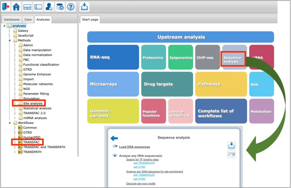
The TFBS prediction tools are located in the Analyses –> Methods –> Site analysis section of the platform, as well as in the Analyses –> Workflows –> TRANSFAC section of the platform. Selected tools for sequence analysis can be found under the Sequence analysis button of the platform start page:

You can find information on the profile selection (collection of positional weight matrices – PWMs – transcription factor binding models that will be used for performing the site search) in this document or in tabular format here.

Search for TF binding sites with TRANSFAC®

The Search for TF binding sites with TRANSFAC® workflow in the geneXplain platform is designed to search for putative transcription factor binding sites, TFBS, in any input DNA sequence in EMBL, Fasta or Genbank formats. Using this workflow you can analyze DNA sequences of any species and of any genomic regions. In the analysis results of this workflow you will find a summary table and a track with found sites in the input sequences.

The summary table gives the site density per thousand bp for each matrix in the input sequence:

Each row summarizes the information for one site model (PWM – positional weight matrix).

For each row, the column Site density per 1000bp shows the number of matches normalized per 1000 bp length for the sequences in the input set.

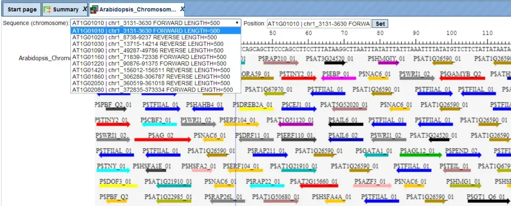
The track of found sites can be visualised in genome browser:

In the field Sequence (chromosome) you can find a dropdown menu. This feature helps to easily switch between visualizations of the sequences in the input set. In this particular example the input sequence set comprises ten individual promoter sequences, and each individual promoter can be visualized in the genome browser.

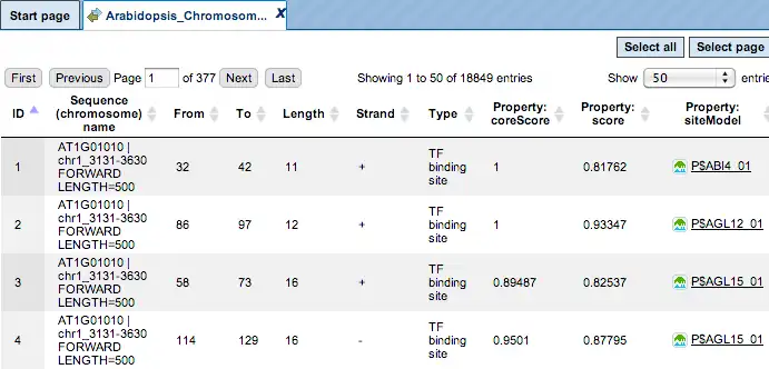
The same track of found sites can be opened as a table for tabular visualisation:

Each row of such table corresponds to one resulting TFBS and includes sequence names, site positions calculated by the algorithm and a site model (TRANSFAC® matrix). This table can be exported as a track in several different formats including intervals, bed, wig and more. DNA sequences can be exported in multi-FASTA format.

Additional visualisation options are available for selected rows of the Summary table: the Report on selected matrices button at the top menu panel of the platform will visualize the found TFBS in the input sequences. In this example, all matrices with a site density <5 were selected. The visualization results are shown below:

There are ten rows corresponding to the individual sequences in the input set. The column Sites view schematically represents the sequence length with mapped TFBSs. Matches for different matrices are shown in different colors. You can select individual matches by mouse click and get additional information in the Info box.


Analyze any DNA sequence for site enrichment with TRANSFAC® 


The Analyze any DNA sequence for site enrichment with TRANSFAC® workflow in the geneXplain platform is designed to search for enriched TFBS in any input DNA sequence as compared to a background DNA sequence. The central part of this workflow is performed by two individual methods: Site search on track and Site search result optimization, both can be found in Analyses –> Methods –> Site analysis.


With this workflow you can analyze sequences of any species and any genomic region.


The input Yes and No sequence sets can be in EMBL, FASTA or GenBank format.


The analysis results of this workflow include several tables and tracks.

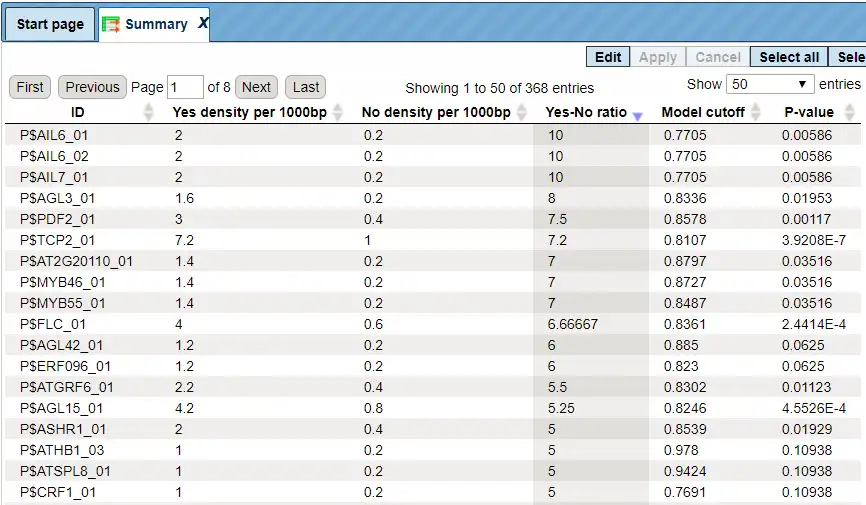
The Summary table provides the overview of the TFBS enriched in the Yes set as compared to the No set:

Each row summarizes the information for one site model (PWM – positional weight matri).


For each row, the columns Yes density per 1000bp and No density per 1000bp show the number of matches normalized per 1000 bp length for the sequences in the input Yes set and input No set, respectively. The Column Yes-No ratio is the ratio of the first two columns. The higher the Yes-No ratio, the higher is the enrichment of matches for the respective matrix in the Yes set. The matrix cutoff values as they are calculated by the program at the optimization step are shown in the column Model cutoff, and the last column shows the p-value of the corresponding event.


TFBSs can be further visualized in the Yes sequences by selecting one or several rows of the Summary table and clicking on the Report on selected matrices button at the top menu panel of the platform.


In this example, all matrices having a Yes-No ratio>3 were selected. The visualization results are shown below:

There are four rows corresponding to the individual sequences in the input Yes set. The column Sites view schematically represents the sequence length with mapped TFBSs. Matches for different matrices are shown in different colors. You can select individual matches by mouse click and get additional information in the Info box.

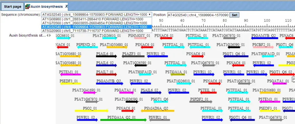
The track of found sites represents TFBSs that are over-represented in the Yes sequences versus the No sequences. It can be viewed in the genome browser:

In the field Sequence (chromosome) you can find a drop down menu. This feature helps to easily switch visualization between the sequences in the input set. In this particular example the Yes sequence set comprises four individual promoter sequences, and each individual promoter can be visualized in the genome browser.


The track of found sites that are over-represented in the Yes sequences versus the No sequences can also be viewed as a table, scores of the putative TFBS are optimized by the algorithm:


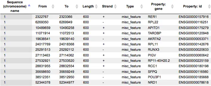
Each row of this table corresponds to one resulting TFBS, and includes its position in the Yes sequences (the columns From and To), length and strand, as well as a score calculated by the algorithm and a site model (matrix). This table can be exported as a track, in several different formats including intervals, bed, wig and more. DNA sequences can be exported in multi-FASTA format.


In case of analysis Human, Mouse or Rat data, as well as since recent release the Arabidopsis, Zebrafish, Nematoda, Fruit fly, Baker’s yeast, and Fission yeast data, additional tables will be outputted by the workflow: Transcription factors Ensembl and Transcription factors Entrez. These tables aim at showing transcription factors linked to the identified site models (matrices). These are potential candidate regulators of genes in the input Yes set. They are supposed to regulate transcription of Yes-genes via the identified enriched TFBSs.

You will find a much more detailed description of the sequence analysis workflows in the geneXplain platform in the respective chapter of the user manual.

Site search on gene set


The Site search on gene set method of the geneXplain platform provides you with an ability to search for putative TFBS in a set of genes. As input for the analysis two gene sets should be provided: Yes (e.g. differentially expressed in an experiment, test set) and No (set of background genes, control set) as well as positional range relative to the TSS and a collection of predefined weight matrices with a particular threshold (profile). The analysis can be done for Human, Mouse, Rat, Arabidopsis, Nematoda, Zebrafish, Fruit fly, Baker’s yeast, and Fission yeast genes.


The Site search on gene set analysis results contain one Summary table and six tracks: yes promoters, no promoters, yes sites, no sites, yes sites optimized, and no sites optimized.


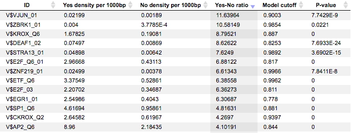
An example of the summary table is shown below:

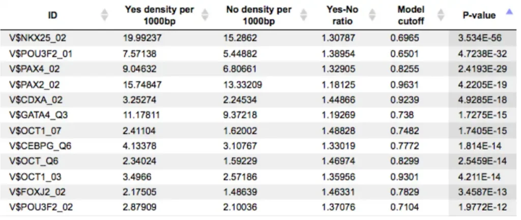
Each row summarizes the information for one PWM. For each selected matrix, the columns Yes density per 1000bp and No density per 1000bp show the number of matches normalized per 1000 bp length for the sequences in the input Yes set and input No set, respectively. The Column Yes-No ratio is the ratio of the first two columns. Only matrices with a Yes-No ratio higher than 1 are included in the summary table. The higher the Yes-No ratio, the higher is the enrichment of matches for the respective matrix in the Yes set. The matrix cutoff values as they are calculated by the program at the optimization step are shown in the column Model cutoff, and the last column shows the p-value of the corresponding event.


The Yes promoters and No promoters tracks represent promoters of the input gene sets. These tracks can be opened as tables:

This table lists the positions of the promoter areas selected for the analysis on particular chromosomes, as shown in the columns From and To. The column Strand shows the strand on which each particular promoter is located. This track can be dragged and dropped on a particular chromosome opened in the genome browser to visualize the localizations of the promoters.

The track Yes sites optimized visualizes those putative sites that are over-represented in the promoters of the Yes set versus the No set as they are located in the promoters of the Yes set. Putative TFBS are shown as a track, scores of the putative sites are optimized by the algorithm.

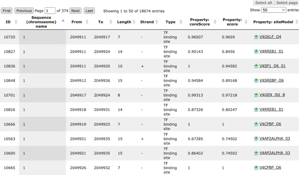
This track is a list of all putative TFBS found in one analysis, it can be opened as a table. Each row presents details for each individual match for every PWM. The columns Sequence (chromosome) nameFromToLength and Strand show, correspondingly, genomic location of the match including chromosome number, start and end positions, strand and length of the match.

The column Type contains information about the type of the elements, in this case all matches are considered as “TF binding site”. Further columns keep information about PWM producing each match (column Property: matrix) as well as score for the whole matrix (column Property: score). The column Property: siteModel contains the identifier for the corresponding site model, which is the matrix together with a cutoff applied (and in the example shown is identical to the matrix identifier).

Yes (No) sites tracks are very similar in structure. The major difference is that these tracks include putative binding sites before the cutoff optimization, and thus they contain more sites.


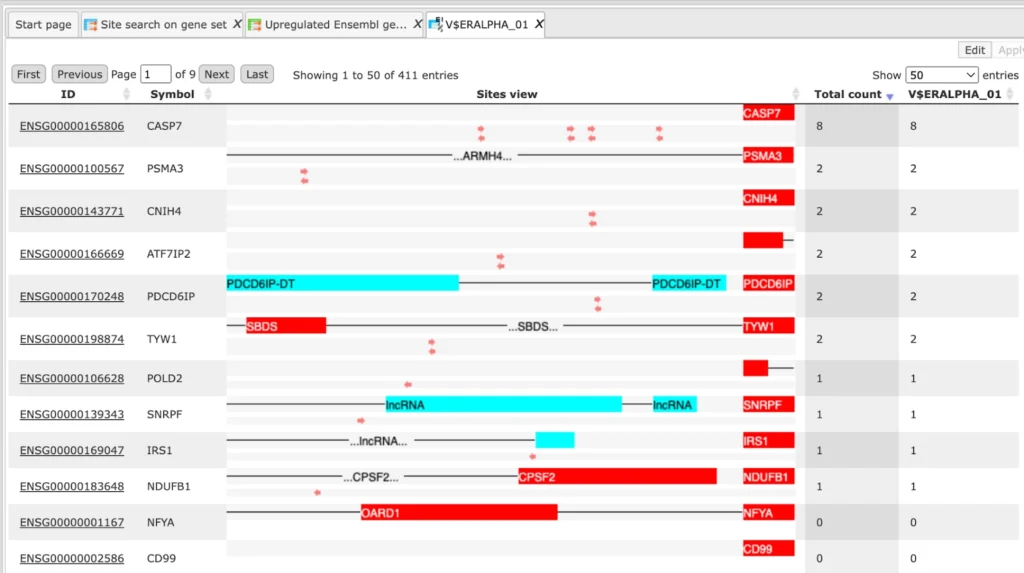
Additional visualisation options of found TFBS are available for individual genes and individual matrices. Different rows of the summary table can be selected and visualized using the “report on selected matrices” button from the top menu panel of the platform: 

This action will open two new files: a table and a track. The constructed track has the same structure as described above for other track files. Each row of the constructed table corresponds to one individual gene:

The column ID presents the Ensembl ID for each gene, and the gene symbol is shown in the column Symbol. The column Sites viewshows a schematic representation for each gene, where blue bars correspond to gene starts and coding regions, and TFBSs for different matrices are shown by arrows of different colors. The column Total count shows the number of TFBSs for all matrices together in the promoter of each particular gene. The next columns are named as matrices in the summary table and represent the number of TFBSs for each matrix in each particular gene.

On the picture above the table is sorted by the column Total count, and on the top we can see those genes that contain the highest total number of sites. This table can be sorted by different columns corresponding to individual matrices, and then on the top you will see those genes that contain the highest number of sites for the matrix in focus. The TFBS color schema in this table can be customized. This table can be exported in tab-separated format (txt) or comma-separated format (csv).

A much more detailed description of the Site search on gene set method can be found in the respective chapter of the geneXplain platform user guide.

Site search on track

The Site search on track method of the geneXplain platform provides you with an ability to search for putative TFBS in an input track. As input for the analysis the track for performing the site search should be provided (e.g. the track of promoter regions of studied genes), as well as the sequence source of the track and the collection of binding models (PWMs) that should be used for the TFBS search.

The result of this method is the track of found sites, which can be visualized as a table:

Each row of the table presents details for each individual match for every PWM. The columns Sequence (chromosome) nameFromToLength and Strand show, correspondingly, genomic location of the match including chromosome number, start and end positions, strand and length of the match. The column Type contains information about the type of the elements, in this case all matches are considered as “TF binding site”. Further columns keep information about PWM producing each match (column Property: siteModel) as well as a score of the core (column Property:coreScore) and a score for the whole matrix (column Property: score). For details about these scores, please see Kel, Alexander E., et al. “MATCH: a tool for searching transcription factor binding sites in DNA sequences.” Nucleic acids research 31.13 (2003): 3576-3579, LINK.

Combinatorial analysis (AI and ML)
Composite modules

Composite modules are combinations of several TFBSs that are found together in a set of regulatory sequences. We search for such combinations of TF binding sites that are overrepresented in the regulatory sequences under study compared to a background set of sequences. The search for composite modules can be performed in the geneXplain platform using our in-house implementation of a genetic algorithm called Composite Module Analyst [Waleev, T., et al. “Composite Module Analyst: identification of transcription factor binding site combinations using genetic algorithm.” Nucleic acids research 34.suppl_2 (2006): W541-W545. Link].

As input for the genetic algorithm we take the output of a site search analysis. There are two individual analysis functions available in the geneXplain platform:
Construct composite modules analysis – this method works on the promoter sequences specified relative to TSS in the set of genes. As input, it takes the results of the Site search on gene set analysis function.

Construct composite modules on tracks – this method works with any DNA sequences specified by their absolute genomic positions, and is very often applied for the analysis of ChIP-seq fragments. As input, it takes the results of the Site search on track analysis function.
they are different with respect to the type of sequences where the search for composite modules is done, and correspondingly with respect to the format of the input data.

Both analysis functions can be found in the Analyses –> Methods –> Site analysis section of the geneXplain platform.
A brief overview of the site search methods (Site search on gene set and Site search on track) that serve as input for the composite modules construction analyses was provided above.

Construction of composite modules

The Construct composite modules method enables the identification of combinations of several TFBSs in the promoters of the genes under study (Yes-set). The resulting composite module differentiates the Yes-set from a background set (No-set). This analysis should be launched on the results of Site search on gene set analysis with the selected Yes-set, No-set and a specified profile of matrices.

The Construct compossite modules on tracks method is designed for identifying combinations of several TFBS in DNA sequences specified by their genomic positions (tracks). An example of a track that is very often used is a set of the ChIP-seq data. The resulting composite module differentiates between a Yes-track and a background (No-track). This analysis should be launched on the results of Site search on track analysis with the selected Yes-set, No-set and a specified profile of matrices.

Details on how to launch these analyses can be found in the respective chapter of the geneXplain platform user guide.

Hierarchical structure of the composite modules

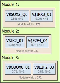
Prior to going into the composite modules analysis results visualisation, we first provide an overview of how the composite modules are visualized. Composite modules may have a complex hierarchical structure consisting of two levels: site models and modules. The highest hierarchical level contains several modules and corresponds to the promoter model.

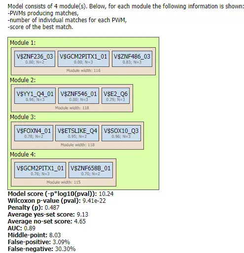
The first level, site model, corresponds to the individual site model, often based on one PWM. Names of the site models are often the same as the matrix names (in case the site models are based on a library of matrices). The site models are taken from the profile that was used in the site search. In the resulting schemas the site models are shown by blue boxes, for instance:

Within these boxes, there are two values below the site model. The first value is the threshold value for the score of the respective site model, which is determined by the genetic algorithm during the optimization process (here it is equal to 0.81); in some cases this value is equal to 0.0, which means that the original threshold value given in the profile was found by the algorithm to be the optimal one. The second value, in this example N=2, is the maximum number of best found individual matches (sites) for this site model which are taken into account for calculating the score of the module.

The next level, module, may contain several site models, shown within the light brown boxes:

The module is characterized by its width, the average length of DNA window containing matches for the mentioned site models. In the example, the module width is 237 bp. In the resulting schemasmodulesare shown in green boxes, and they are numbered, e.g. Module 1, Module 2, ….

In the input form you can define the complexity of the promoter model to be constructed by specifying the number of units of each level: number of modules, number of site models, and also the minimum and maximum numbers of individual sites to be considered.

For example, in the visualisation below the number of modules was specified from 2 to 3, and correspondingly the resulting promoter model contains three modules: Module 1, Module 2, and Module 3. The number of site models was specified from 2 to 2, which means that the search was performed for pairs of individual site models. Respectively, in the resulting image you can see that each module contains two site models highlighted by blue circles:

Construct composite modules results visualization and interpretation

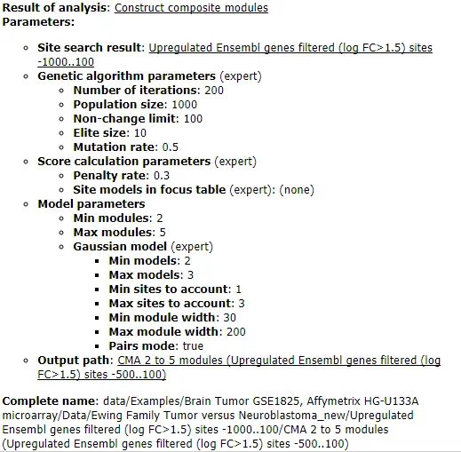
Below we provide the results visualisation of the Construct composite modules analysis obtained for the demo input data set. The input parameters of the method that were used for the analysis launch were as follows:

As a result, the method constructed two tables (Model visualization on Yes set and Model visualization on No set), two tracks (Yes track and No track), and one histogram.


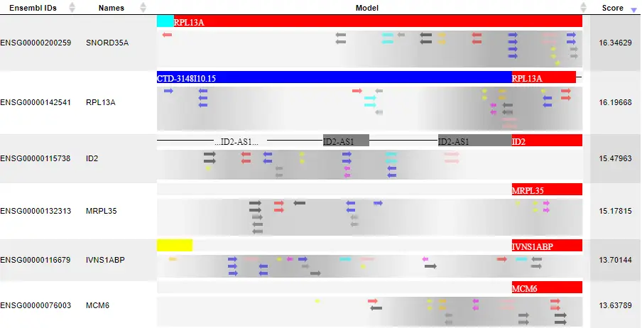
In the Model visualization on Yes set table the the primary results of the analysis are presented: the identified composite modules are shown in the promoters of the Yes set:

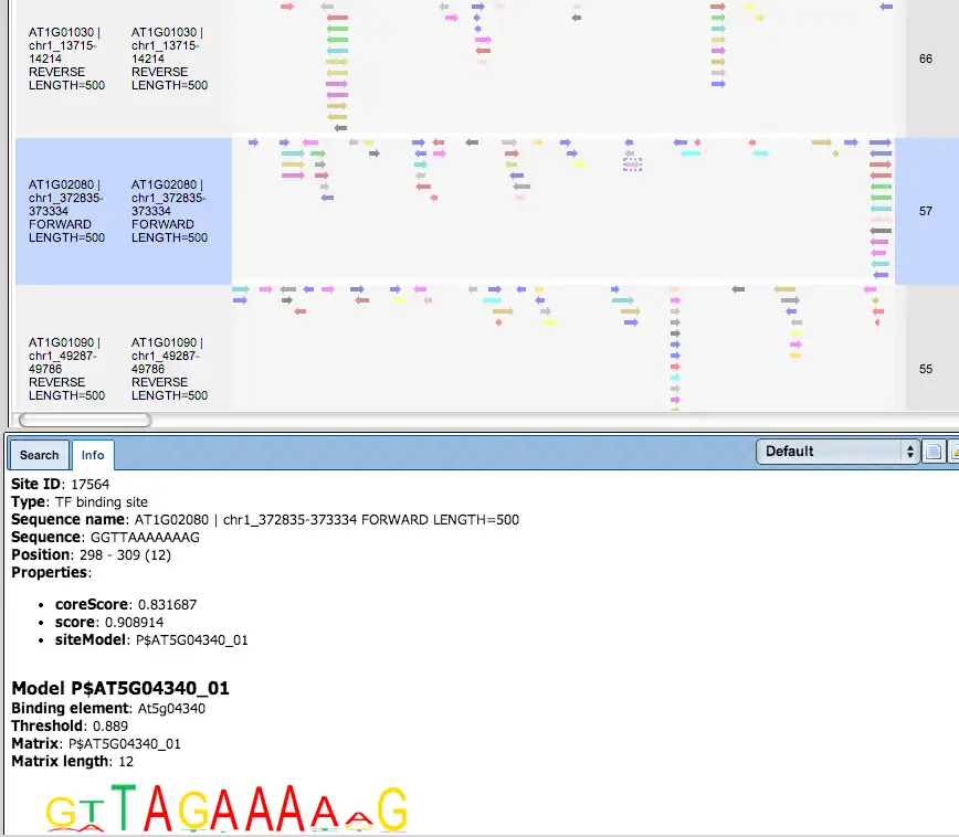
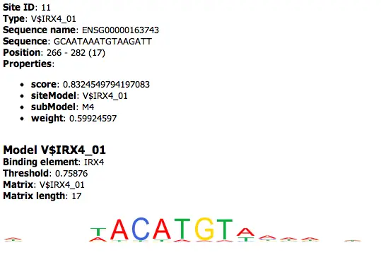
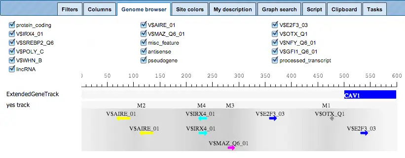
Each row in this table corresponds to one gene of the Yes set, and for each gene the Ensembl ID and the gene symbol are shown in the two first columns. The column Model displays a symbolic map of the gene promoter taken for the analysis, in this case -500/+100 relative to the TSS. Arrows of different colors correspond to individual TFBSs, and a gradient in grey corresponds to the statistical density of the identifiedcompositemodules. The most intensive grey color corresponds to the center of a composite module. Each individual TFBS on this map is clickable, and upon a click information is displayed in the Info box (bottom left corner in the tool). As an example, one blue arrow is selected on the promoter of the top gene in the screenshot above, and for this selected TFBS the following details are shown in Info box:

The last column in the table, Score, shows a score calculated for each promoter depending on the number of modules, site models, sites, their scores and other statistical parameters. The higher the score for a promoter, the better the differentiation of this promoter from the promoters of the No set. The column Score is used for default sorting of the table, with the highest scores on top.

In addition to that, at the bottom part of the tool in the Model visualization on Yes set table you can also see the schematic representation of the hierarchical structure of the identified composite module, as well as a comprehensive set of its statistical characteristics:

The Yes track provides essential information about the regulation of individual promoters and is therefore important to be included in the visualization of individual promoters by the genome browser.


The schematic visualization can be comfortably extended to a more detailed visualization for each individual promoter:

For a selected promoter, you can see a more detailed map, including the names of the matrices and the numbers of individual modules, M1 through M4. Each element of this interactive map has a corresponding check box. Unchecked elements will not be displayed on the map. De-selection is applied simultaneously to both: the detailed view of one promoter, and the table with the schematic representation of all promoters.

The table Model visualization on No set shows a visualization of the identified composite modules in the promoters of the No set.
The structure of this table is the same as that of the Model visualization on Yes set table, described above.

The function of the No track is to provide a possibility for a detailed visualization of no promoters in a way similar to that of the Yes track.

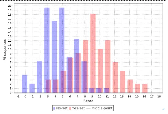
The distribution of scores for individual promoters is shown as a Histogram, where the promoter score value is shown on X axis and the percentage of promoters (% sequences) having this score is shown on the Y axis:

This histogram can be further interpreted applying the statistical characteristics described above.

The center, a vertical grey line, corresponds to the average score value and is equal to 3.44 in this example. Promoters from the No set with a score above 3.44 are shown in the histogram as blue bars to the right of the center, and they are referred to as false positives. In this example, the false positive rate is 16.82 %.

Promoters from the Yes set with a score below 3.44 are shown in the histogram as red bars to the left of the center, and they are referred to as false negatives. In this example, the false negative rate is 23.42 %.

A visual analysis of the histogram suggests that the Yes promoters with a score above 4.5 are very well separated from the No promoters, which means that for this part of the promoters the composite model constructed is most suitable. In this example there are 38 promoters with the score value >4.5; they can be saved as a separate gene set, and for them the model obtained works best.

Score calculation of the composite models

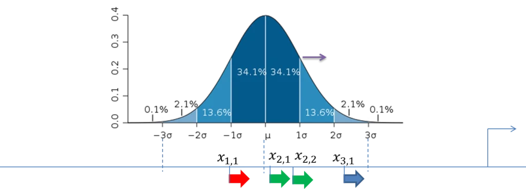
The figure below demonstrates the calculation of the score value for the composite modules in the promoter sequences. The TSS is shown as a thin arrow on the right side of the figure. Four thick arrows exemplify four sites found in this promoter. The color of the arrows exemplifies the site model which these sites belong to (three site models – red, green and blue).

A promoter model consists of modules. The score of each module Mk(Score(Mk),k= 1, …,K) is calculated according to this formula:

Here, Site Score (t,i) is the site score for the sites found in the promoter, which is calculated by the Match algorithm.

mt– the number of sites of the site model found in the promoter.

Tk– the number of site models in the module Mk, and

The final promoter score is calculated as the sum of the module scores Mk.

Standard deviation (σ) of the normal distribution is subject of optimization by the genetic algorithm and represents the width of the module in the output of the composite module analysis.

Further details on the composite modules construction can be found in the respective chapter of the geneXplain platform user guide.

Combinatorial models based on sparse logistic regression (MEALR)

Combinatorial regulation analysis of genomic or custom sequences

This workflow scans input sequences for types of transcription factor binding regions represented in the library of MEALR models enclosed with TRANSFAC®. It is primarily intended to be applied for single sequence analysis.

The workflow proceeds through the following main steps.

  1. Prediction of potential binding locations using the TRANSFAC® MEALR combinatorial regulation analysis
  2. Extraction of TRANSFAC® PWMs represented by MEALR model hits using the Extract TRANSFAC® PWMs from combinatorial regulation analysis
  3. Preparation of a cutoff profile with extracted PWMs for subsequent MATCHTM search using the Create profile from site model table
  4. Prediction of binding sites represented by PWMs in input sequences using the TRANSFAC® MATCHTM for tracks
  5. The tools Filter track by condition and Intersect tracks are applied to derive filtered model predictions and intersections of predicted TF binding site and combinatorial model locations.

Prediction of functional transcription factor (TF) binding sites is a difficult task, because recognized DNA elements are rather short (typically between 10 and 20 base pairs) and often do not follow simple rules with regard to sequence specificity. Formation of TF-DNA complexes depends on a context determined by intertwining conditions like cellular differentiation, chromatin state, or expression and activity of cooperating TFs.

With almost 1000 human TFs, over 300 cell types and more than 50 tissue types, the TRANSFAC® library of MEALR models provides the first comprehensive collection of TF binding models that account for combinatorial TF-DNA complexes comprising multiple DNA-binding specificities as well as cellular and tissue-related contexts. These models can therefore deliver predictions with increased accuracy, so that subsequent searches for binding sites that mark the locations of individual TFs are able to focus on relevant PWMs. This is an important step to select from the large number of PWMs curated by TRANSFAC® and to prioritize binding sites of interest. Within longer sequences the MEALR model predictions furthermore suggest subregions where binding by certain TFs most likely occurs.

A much more detailed description of this workflow can be found here.

MEALR combinatorial regulation analysis

This analysis applies combinatorial regulatory models (CRMs) based on the MEALR affinity score [1] to classify or scan sequences for occurrences of combinations of transcription factor binding sites represented by TRANSFAC® PWMs. The models are taken from the MEALR library whose training data originate from the TRANSFAC® collection of high-throughput sequencing experiments.

The method can be launched either in a classification or in the scan mode. The Classification mode evaluates input sequences as a whole, whereas the scan mode analyzes sequence windows separated by the given step size (sliding window). In scan mode, the Best hit method reports the best scoring sequence window disregarding a cutoff and the Cutoff method reports the best non-overlapping windows satisfying the specified cutoff.

The output folder encompasses a table and sequence track with information about model hits. The output table contains sequence start and end points of hits, model ids, match probabilities as well as other values as described below. For input sequences derived from genomic regions (instead of imported as custom sequences) the table includes in addition a sequence id generated for a region as well as the genomic sequence id, start and end coordinates.

[1] Katie Lloyd, Stamatia Papoutsopoulou, Emily Smith, Philip Stegmaier, Francois Bergey, et al., The SysmedIBD Consortium; Using systems medicine to identify a therapeutic agent with potential for repurposing in inflammatory bowel disease. Dis Model Mech 1 November 2020; 13 (11): dmm044040.

A much more detailed description of this mathod can be found here.

Extract TRANSFAC® PWMs from combinatorial regulation analysis

This tool extracts TRANSFAC® PWMs from a result table generated by the MEALR combinatorial regulation analysis. The PWMs represent transcription factor binding specificities that constitute the combinatorial module predicted by the MEALR model.

The output contains the TRANSFAC® PWMs extracted from MEALR models according to specified cutoffs. This table can further be applied in several analyses, e.g. to extract corresponding transcription factors using the tool or to create a profile for binding site predictions ( Create profile from site model table) with MATCHTM.

A much more detailed description of this mathod can be found here.

Mapping TFBS on peaks calculated from ChIP-seq data

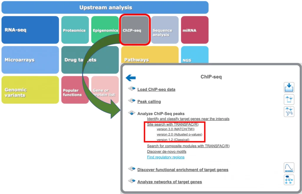
The geneXplain platform also provides tools for mapping of TFBS to the peaks calculated from ChIP-seq data. You will find respective workflows under the ChIP-seq button of the geneXplain platform main menu:

Site search in ChIP-seq peaks: Version 1.2 (Classical)

This workflow helps to map TFBS on peaks calculated from ChIP-seq data. Site search is done with the help of the TRANSFAC® library of positional weight matrices, PWMs, using the pre-computed profile vertebrate_non_redundant_minSUM.

The input track should be provided in the BED format and submitted to the analysis as the Yes track. The No track can be selected from the ready tracks of housekeeping genes or uploaded as a custom track of your choice.

The results of the workflow contain two tables: Site optimization summary and Transcription factors and two tracks: Yes sites opt and No sites opt.

The Site optimization summary table includes the matrices the hits of which are over-represented in the Yes track versus the No track. Only the matrices with Yes-No ratio higher than 1 are included in this output table. The hits of these matrices can be interpreted as over-represented in the Yes set versus No set:

Each row of this table summarizes the information for one PWM. For each selected matrix, the columns Yes density per 1000bp and No density per 1000bp show the number of matches normalized per 1000 bp length for the sequences in the input Yes set and input No set, respectively. The Column Yes-No ratio is the ratio of the first two columns. Only matrices with a Yes-No ratio higher than 1 are included in the summary table. The higher the Yes-No ratio, the higher is the enrichment of matches for the respective matrix in the Yes set. The matrix cutoff values as they are calculated by the program at the optimization step are shown in the column Model cutoff, and the last column shows the P-value of the corresponding event.

The Transcription factors table includes transcription factors (TFs) that are associated with the PWMs that are listed in the table Site optimization summary:

Each row of this table shows details for one TF, including its Ensembl gene ID (column ID), gene symbol, gene description and biological species of the corresponding TF (columns Gene descriptionGene symbol, and Species). The column Site model ID shows the identifier of the PWM associated with this TF, and several further columns repeat information that is also shown in the table Site optimization summary.

Each row of the tracks Yes sites opt and No sites opt presents details for each individual match for every PWM:

Columns Sequence (chromosome) nameFromToLength and Strand show the genomic location of the match including chromosome number, start and end positions, strand and length of the match, respectively. The column Type contains information about the type of the elements; in this case all matches are considered as “TF binding site”. Further columns keep information about PWM producing each match (column Property:matrix) as well as a score of the core (column Property:coreScore) and a score for the whole matrix (column Property:score). The column Property: siteModel contains an identifier for the site model, which is the matrix together with the cutoff applied (for details about these scores, please see Kel, Alexander E., et al. “MATCH: a tool for searching transcription factor binding sites in DNA sequences.” Nucleic acids research 31.13 (2003): 3576-3579, LINK.

The genome browser visualization of the constructed tracks is shown below:

Such a view may help to visually co-localize information on different tracks, e.g. putative TFBS with variations, repeats and genes. In the figure above, the cursor shows position 29444, and two variations are located at this position. You can immediately recognize that these variations are located within particular putative binding sites in the intron region of the WASH7P gene.

The same information is available not just as a picture, but also as a table. For each element information is shown on chromosome, positions, length, strand, type of the track, and name of the element:

This table can be exported as a track, in several different formats including intervals, bed, wig, gff, gtf and more.

The same workflow can be launched on multiple interval sets: in the input Yes tracks field several different tracks can be simultaneously submitted. The same background dataset, Input No track, is used for comparison with each of the submitted Yes tracks. The default No track corresponds to far upstream regions of the house keeping genes, where no functional TFBSs are expected. The workflow will iteratively perform the same steps for each of the input Yes tracks. This helps to save time and efforts, especially when you have several sets of ChIP-seq data, e.g. the peaks for a number of different TFs.

A much more detailed description of this workflow can be found here.

Site search in ChIP-seq peaks: Version 2.0 (Adjusted p-values)

This workflow is designed to map putative enriched TFBSs on peaks calculated from your ChIP-seq data (Yes set) as compared to a random background set (No set). Importantly, the No set is created automatically and contains by default 1000 intervals. In the first part of the workflow, the enriched motifs are identified by our proprietary MEALR approach.

Enriched motifs serve as a basis to construct a specific profile. At the next step this newly generated profile is run on the same list of input peaks applying the search for enriched TFBSs on tracks method.

The input track should be provided in the BED format as the Input Yes track – it is the track with peaks from your ChIP-seq study.

Select the profile (collection of PWMs to perform the search for TFBS) – vertebrate_non_redundant_minSUM by default (any other TRANSFAC® profile or custom user-specific profile can be selected).

A filter for the coefficient of the MEALR method should also be specified. The default filter is set as >0.125 to have 75% or more of true discovery rate, TDR. For 90% TDR, you can type 0.270 in this field and for 50% TDR – 0.05593. The filtered motifs are included in the output asenriched motifs. At the later step, PWMs corresponding to the enriched motifs are used to make a new profile.

In the results of the workflow you will find four tables (Enriched motifs MEALR, Transcription factors, Site search summary, Profile) and three tracks (Random No sites optRandom No track and Yes sites opt filtered track), the folder with demo results of this workflow can be viewed here.

The table Enriched motifs MEALR includes enriched motifs in the Yes track versus the No track, filtered by the coefficient as specified.

Please note that by default only the matrices with a Coefficient > 0.125 (75%TrueDiscoveryRate) are included in this output table. These motifs can be interpreted as the best discriminating motifs between the Yes and No sets.

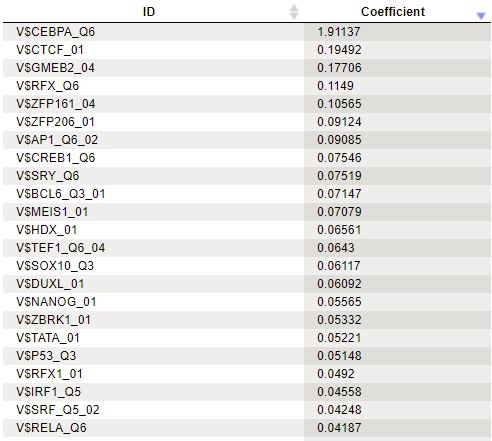
The table Enriched motifs MEALR shown below has been sorted by the values in the Coefficient column. The larger the coefficient, the more important the corresponding motif was for discriminating between Yes and No sequences:

The table Profile is opened automatically and is an input-specific profile, based on the filtered enriched motifs MEALR:

This profile is an intermediate result of the workflow and is used further for Site search on gene set analysis in the second part of the workflow.

The Transcription factors Ensembl table includes transcription factors (TFs) that are associated with the PWMs listed in the table Site search summary:

Each row of this table shows details for one TF, including its Ensembl gene ID (column ID), gene symbol, gene description and biological species of the corresponding TF (columns Gene description, Gene symbol, and Species). The column Site model ID shows the identifier of the PWM associated with this TF, and several further columns repeat information that is also shown in the table Site search summary.

A much more detailed description of this workflow can be found here.

Site search in ChIP-seq peaks: Version 3.0 (MATCH (TM))

This workflow is designed to search for enriched transcription factor binding sites (TFBSs) in a set of genomic sequences in comparison to a random background set. With this workflow you can analyze sequences from the genome of human, mouse, rat, arabidopsis or zebrafish. To identify enriched binding sites within the sequences, positional weight matrices from the TRANSFAC(R) database are used while performing the method TRANSFAC(R) MATCH(TM) for tracks. The site search result will be further converted into a table of potential transcription factors that can bind to the identified TFBSs. The identified enriched transcription factor binding sites can be visualized in the genome browser.

Genomic sequences in track format (input example) can be submitted for the input. A random track of 1000 sequences that does not overlap with the input sequences is automatically generated as the background set.

The results of the workflow contain several tables and tracks. The identified enriched transcription factor binding sites (TFBSs) are present in a summary table (result example) and can be visualized in the genome browser as a track (result example). The potential transcription factors are given in a final Ensembl table (result example) with annotated GeneSymbol IDs and a short description.

A much more detailed description of this workflow can be found here.

Search for composite modules on ChIP-seq peaks with TRANSFAC®

This workflow finds pairs of TFBSs that discriminate between two tracks, theYes and the No tracks. As the Yes track, the ChIP-seq peaks identified as binding profiles for particular transcription factors can be considered.

The ChIP-seq experimental technology is widely applied to a variety of biological problems, in particular to study genome-wide histone modification profiles, e.g. histone methylation and histone acetylation profiles. Correspondingly, the same workflow in the platform can be used to analyze histone modification profiles as well.

For an example let’s consider the results of the workflow application to find composite modules in the ChIP-seq peaks identified for in-vivo-bound fragments of transcription factor E2F1 in HeLa cells, published in Gene Expression Omnibus,GSM558469.

Input Yes track. The original track of genome-wide E2F1 binding fragments was filtered by the length shorter than 600 bp, which resulted in 249 fragments. This track of 249 fragments is used as the input Yes track. The track can be found here.

Input No track. A track of the far upstream fragments of the human housekeeping genes located on chromosome 1 is taken as the No track. The track can be found here.

The results of this analysis run can be found here.

The results contain the Site optimization summary table, which contains those site models that are over-represented in the Yes track as compared to the No track:

Each row of the table represents the result for one PWM from the input profile. Only those PWMs with Yes-No ratio >1 are included in the output. Upon sorting by the Yes-No ratio, matrices for E2F factors are among top 20 lines. Please note that the p-values of E2F matrices are extremely low, which demonstrates highest statistical significance of the results.

The Modules folder in the results of the workflow contains the found composite module. The composite module found on our example contains two pairs, and we can see by exactly which site models (matrices) these pairs are formed as well as the statistical parameters of the overall model. Both pairs contain matrices for E2F factors:

For further details on this workflow and its results interpretation please refer to the respective chapter of the geneXplain platform user guide.

Search for discriminative sites with TRANSFAC® (MEALR)

The tool MEALR finds combinations of TFBS matrices that discriminate between two sets of sequences (denoted asYes and No sets). TheYes set may consist of genomic regions identified in a ChIP-seq experiment. No sequences are often other non-coding genomic regions not overlapping with the peaks.

MEALR differs from other tools in the following points:

  • No cutoff or threshold is used on matrix scores to determine potential binding sites. Instead, MEALR calculates threshold-free sequence scores.
  • MEALR builds a discriminative model for classification which is well-established and widely applied in statistical analysis called Sparse Logistic Regression. The model consists of a linear model that estimates the probability that a sequence belongs to the Yes set based on its binding site features.
  • The sparseness constraint enables MEALR to select a subset of matrices relevant for classification of Yes and No sequences from a possibly large matrix library. Therefore MEALR’s output differs from other tools by presenting a focused set of matrices.
  • While other site enrichment tools provided in the platform evaluate enrichment separately for each matrix, the model used in MEALR assesses the importance of matrices for discrimination in combination with other matrices of the library. Therefore, MEALR suggests (linear) combinations of transcription factor motifs.

For each input sequence x MEALR calculates a score for each PWM by the following equation where W denotes the number
of windows scored by the PWM and LSmax(xw) is the high log-odds score of window w :

f(x) = log( Σw exp(LSmax(xw)) / W )

Each sequence is therefore associated with a vector of scores, one from each matrix, and a class (Yes, No).

Let us present an example analysis for a ChIP-seq data set consisting of 500 peak regions and 1000 sequences randomly sampled from regulatory regions across the human genome.

Yes set  is the set of sequence intervals that you want to analyze, for example these can be ChIP-seq peak regions.

No set is the set of background intervals (control set).

In the input profile (collection of PWMs – binding motifs) the cutoffs will be ignored, because MEALR calculates whole sequence scores.

In the results of analysis the summary table would look like this:

A row of this table contains matrix identifier and its logistic regression coefficient. The larger the coefficient value, the more important the corresponding matrix was for discriminating between Yes and No sequences. In our example, three of the five top matrices represent members of the transcription factor subfamily C/EBP.

For further details on this method please refer to the respective chapter of the geneXplain platform user guide.

geneXplain platform: 

TRANSFAC®  is equipped with the best in the field, flexible online software platform that provides: 

Omics analysis: 
It has multiple tools for analysis of practically any omics data, including: RNA-seq, ChIP-seq, ATAC-seq, CUT&RUN, WGS, WES, and many others, also on the single cell level.

Over 200 tools and pipelines:  
It integrates over 200 tools for analysis of gene lists and DEGs, as well as data in hundreds of input formats, such as FASTA, FASTQ, VCF, BED, ect. It is integrated with Galaxy platform and is equipped with a flexible workflow management system providing a variety of ready pipelines in all fields of bioinformatics.    

Easy GUI:  
The geneXplain platform provides a powerful and flexible graphical user interface (GUI) running in the web browser. User don’t need to do any installations and dont require to have any prior programming skills. The platform is the ready solution for no-coding bioinformatics

API: 
An elaborated Application Program Interface is freely available for  geneXplain platform. It is provided for Python, R and Java and can be downloaded here:
https://github.com/genexplain

Cloud Storage: 
100GB of working space is provided for the users of geneXplain platform in TRANSFAC Basic package. Users can use this space for uploading data and storing results in an unlimited number of projects. 

The geneXplain platform is an online toolbox and workflow management system for a broad range of bioinformatic and systems biology applications. The individual modules, or Bricks, are unified under a standardized interface, with a consistent look-and-feel and can flexibly be put together to comprehensive workflows. The workflow management is intuitively handled through a simple drag-and-drop system. With this system, you can edit the predefined workflows or compose your own workflows from scratch.
 
Own Bricks can easily be added as scripts or plug-ins and can be used in combination with pre-existing analyses.
GeneXplain GmbH provides a number of state-of-the-art bricks; some of them can be obtained free of charge, while others require licensing for small fee in order to guarantee active maintenance and dynamic adaptation to the rapidly developing know-how in this field.
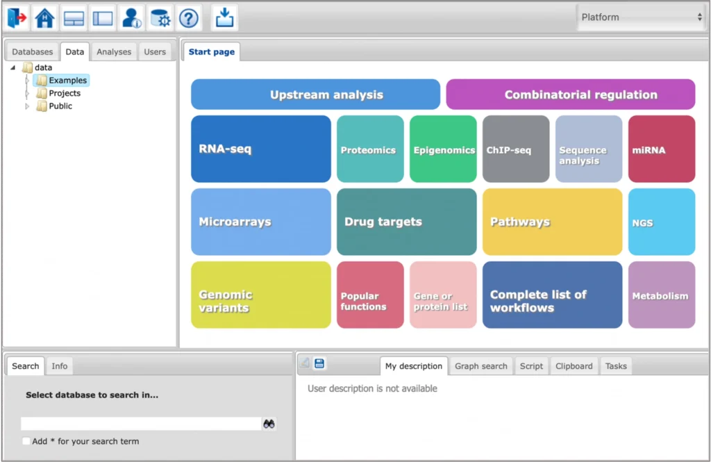
The start page provides an easy access to a number of application areas.

Key features
Integrated AI and ML tools for TFBS prediction

The platform provides access to advanced tools for prediction of genomic transcription factor (TF) binding sites and composite regulatory regions using such algorithms of Machine Learning (ML) and Artificial Intelligence (AI) as Genetic Algorithms and Sparse Logistic Regression.

Integrated databases and analysis tools

The platform provides an integrated view on several databases and analysis tools, public domain as well as commercial ones. They can be combined in a highly flexible way to design customized analyses.

Ready-made workflows for an easy start

A rapidly growing number of proven workflows facilitates a quick and easy access to the platform and its complex analysis functions. Input forms are simple and user-friendly. Workflows can be easily customized to specific needs. Experienced users can create their own workflows.

Fully integrated upstream analysis

The platform provides a fully integrated upstream analysis, which combines state-of-the-art analysis of regulatory genome regions with sophisticated pathway analyses.

Knowledge-based data analysis

The platform uses a number of renowned high-quality databases for the data analysis. TRANSFAC® and TRANSPATH® are expert-curated databases. GeneWays is generated by an NLP-based text-mining approach, providing a helpful complement for manually curated data. Well-known public-domain databases like Reactome and HumanCyc are integrated and applied as well.

JavaScript and R scripts

User-specific scripts in JavaScript and in R can be added directly into the platform, and immediately executed. They can be combined with pre-existing analyses, and can be part of the workflows.

NGS data analysis

NGS data analysis is supported by the platform. ChIP-seq data sets containing in vivo transcription factor binding sites or methylation results can be analyzed with the help of ready-made workflows. Galaxy tools are integrated, supporting RNA-seq data analysis, and many functions more.

Simulation engine inside

The platform contains a simulation engine that executes differential equation systems and visualizes the results. Parameter optimization, parameter fitting (based on expression data), and hierarchical modeling are supported.

Group project work including chat function

Share your data and results with other members of the project. Discuss what you are doing while working together on a dataset.

In addition to that, all our customers enjoy the following advantages or our products:

–       Technical and scientific support or your research: rapid answers to your questions from our professional support team will be always provided

–       Secure cloud space connected with online licenses that can be accessed from any location

–       Extensive manuals, documentation, examples, and tutorials available for all our products

–       Frequent releases and updates of our databases contents and software functionality

–       Ability to request personal training sessions

–       All our servers are running on CO2-neutral water or wind power

Insights
RNA-seq data analysis

From raw reads to full integrated & advanced gene analysis of your experimental data.

Transcription factor identification

Find enriched transcription factor binding sites and corresponding factors/enhancers.

Networks and key signaling molecules

Upstream analysis to discover novel master regulators and underlying mechanisms.

Next generation sequencing

Gene expression profiling, detection of genetics changes and molecular analysis.

Drug target assessment

Integrated promoter and pathway analysis to find prospective therapeutic targets.

Pathway enrichment

Identify key nodes and inferred activity in canonical pathways or reconstructed networks.

ChIP-seq data analysis

Calling peaks, find regulatory regions, classify and analyze target genes.

Single Nucleotide Polymorphisms

Identify affected regulatory DNA motifs and find damaged signal proteins.

Gene Ontology

Map, reduce and visualize GO terms to get a functional classification.

Single Sequences in Genome browser

Work with human, mouse, rat, zebrafish and arabidopsis genome builds.

miRNA characterization

Target identification, get binding site enrichment and tissue specificity.

Genomic variants verification

Predict variant effects and get a molecular tumor board report.

New applications

Updated databases

  • TRANSFAC® 2024.2
  • TRANSPATH® 2024.2
  • HumanPSD™ 2024.2
  • Ensembl Human 112 (hg38)
  • Ensembl Mouse 112 (mm10)
  • Ensembl Rat 112 (mRatBN7.2)
  • Ensembl Zebrafish 112 (GRCz11)
  • Ensembl Nematoda 112 (wbcel235)
  • Ensembl Fruit fly 112 (dm6)
  • Ensembl Saccharomyces Cerevisiae 112 (sacCer3)
  • Ensembl Schizosaccharomyces Pombe 112 (ASM294v2)
  • Ensembl Arabidopsis Thaliana 112 (TAIR10)

GO functional classification for model organisms

  • Perform GO-based functional classification of the studied gene set (Human, Mouse, Rat, Zebrafish, Arabidopsis, Nematoda, Fruit fly or Baker’s yeast gene lists are supported)
  • Visualise the results of the functional classification with a colourful tree map

Here are videos about “RNA-seq preprocessing with the geneXplain platform”

Here is a playlist about “RNA-seq data analysis from FASTQ files to master regulators with geneXplain platform”

Find below a compilation of our introductory and tutorial videos

In English Language

This video is a general introduction to the geneXplain® platform. (3:21 min)

This video is about how to convert gene identifiers from Ensembl to others in the geneXplain platform. (3:02 min)

This video is about how to annotate a gene table with the geneXplain platform. (2:57 min)

In Chinese Language

This video is a general introduction to the geneXplain® platform; it introduces you to different workflows. (1:38 min)

It shows you how to register a free platform account and to login. The audio-visual also introduces you to the look and feel of the geneXplain® platform interface. (4:11 min)

This video demonstrates how to upload raw data from an experiment to the geneXplain®platform for further analysis. (2:46 min)

In this video microarray data is used as an example to show you how to further analyze data from high-throughput experiments on the geneXplain® platform. (6:45 min)

Examples

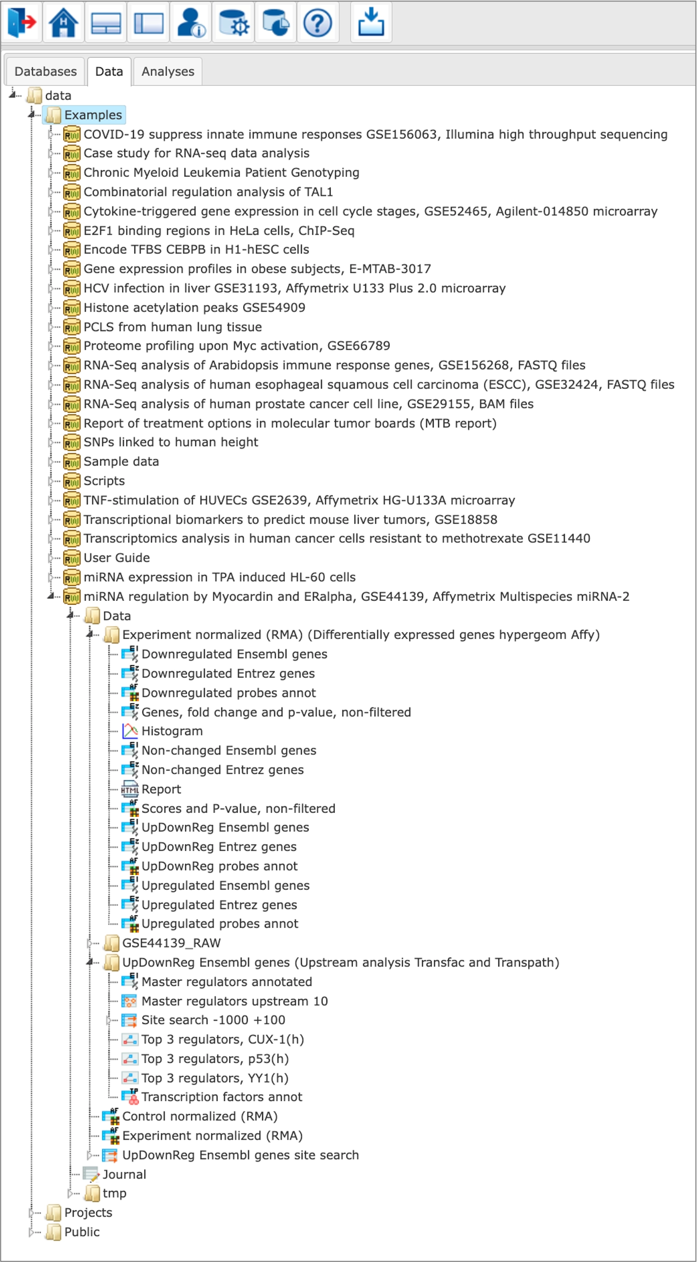
Any user of the geneXplain platform can view the free examples demonstrating the platform abilities towards processing various types of multi-omics data in different studied biological processes and pathologies.

The Examples are located in the Data tab of the geneXplain platform interface under the Examples folder:
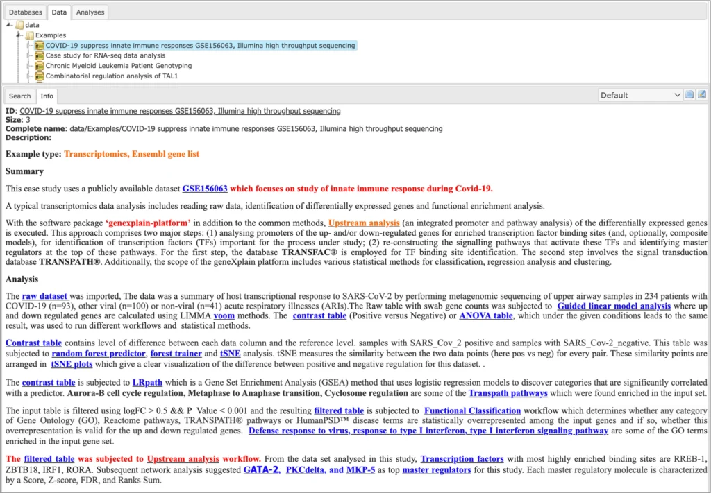
Description of each example is available in the info box upon the click on the name of the respective project:
Publications

Selection of geneXplain platform citations by third-party researchers:

  • Novikova S., Tolstova T., Kurbatov L., Farafonova T., Tikhonova O., Soloveva N., Rusanov A., Zgoda V. (2024) Systems Biology for Drug Target Discovery in Acute Myeloid Leukemia. Int. J. Mol. Sci.  25(9), 4618 Link
  • Kisakol, B., Matveeva, A., Salvucci, M., Kel, A., McDonough, E., Ginty, F., Longley, D., Prehn, J. (2024) Identification of unique rectal cancer-specific subtypes. Br J Cancer. 130, 1809–1818. DOI https://doi.org/10.1038/s41416-024-02656-0. Link
  • Xinxin Liu., Zhihua Huang., Qiuzheng Chen., Kai Chen., Weikang Liu., Guangnian Liu., Xiangyu Chu., Dongqi Li., Yongsu Ma., Xiaodong Tian., Yinmo Yang. (2024) Hypoxia-induced epigenetic regulation of miR-485-3p promotes stemness and chemoresistance in pancreatic ductal adenocarcinoma via SLC7A11-mediated ferroptosis. Cell Death Discovery. 10, 262. Link
  • Drake, C., Zobl W., Wehr M., Koschmann J., De Luca D., Kühne B. A. , Vrieling H. , Boei J. , Hansen T. , Escher S. E. (2023) Substantiate a read-across hypothesis by using transcriptome data—A case study on volatile diketones. Front. Toxicol. 5Link
  • Rajavel A., Klees S., Hui Y., Schmitt A.O., Gültas M. (2022) Deciphering the Molecular Mechanism Underlying African Animal Trypanosomiasis by Means of the 1000 Bull Genomes Project Genomic Dataset. Biology (Basel). 11(5), 742. Link
  • Menck K., Wlochowitz D., Wachter A., Conradi L.C., Wolff A., Scheel A.H., Korf U., Wiemann S., Schildhaus H.U., Bohnenberger H., Wingender E., Pukrop T., Homayounfar K., Beißbarth T., Bleckmann A. (2022) High-Throughput Profiling of Colorectal Cancer Liver Metastases Reveals Intra- and Inter-Patient Heterogeneity in the EGFR and WNT Pathways Associated with Clinical Outcome. Cancers 14(9), 2084. Link
  • Myer P.A., Kim H., Blümel A.M., Finnegan E., Kel A., Thompson T.V., Greally J.M., Prehn J.H., O’Connor D.P., Friedman R.A., Floratos A., Das S. (2022) Master Transcription Regulators and Transcription Factors Regulate Immune-Associated Differences Between Patients of African and European Ancestry With Colorectal Cancer. Gastro Hep Adv. 1(3), 328–341. Link
  • Kawashima Y., Nagai H., Konno R., Ishikawa M., Nakajima D., Sato H., Nakamura R., Furuyashiki T., Ohara O. (2022) Single-Shot 10K Proteome Approach: Over 10,000 Protein Identifications by Data-Independent Acquisition-Based Single-Shot Proteomics with Ion Mobility Spectrometry. J Proteome Res. 21(6), 1418–1427. Link
  • Klees S., Schlüter J.S., Schellhorn J., Bertram H., Kurzweg A.C., Ramzan F., Schmitt A.O., Gültas M. (2022) Comparative Investigation of Gene Regulatory Processes Underlying Avian Influenza Viruses in Chicken and Duck. Biology (Basel). 11(2), 219. Link
  • Benjamin, S.J., Hawley, K.L., Vera-Licona, P., La Vake, C.J., Cervantes, J.L., Ruan, Y., Radolf, J.D., Salazar, J.C. (2021) Macrophage mediated recognition and clearance of Borrelia burgdorferi elicits MyD88-dependent and -independent phagosomal signals that contribute to phagocytosis and inflammation. BMC Immunol. 22, 32. Link
  • Menck K., Heinrichs S., Wlochowitz D., Sitte M., Noeding H., Janshoff A., Treiber H., Ruhwedel T., Schatlo B., von der Brelie C., Wiemann S., Pukrop T., Beißbarth T., Binder C., Bleckmann A. (2021) WNT11/ROR2 signaling is associated with tumor invasion and poor survival in breast cancer. J Exp Clin Cancer Res. 40, 395. Link
  • Meier, T., Timm, M., Montani, M., Wilkens, L. (2021) Gene networks and transcriptional regulators associated with liver cancer development and progression. BMC Med. Genomics 14, 41. Link
  • Chereda H., Bleckmann A., Menck K., Perera-Bel J., Stegmaier P., Auer F., Kramer F., Leha A., Beißbarth T. (2021) Explaining decisions of graph convolutional neural networks: patient-specific molecular subnetworks responsible for metastasis prediction in breast cancer. Genome Med. 13, 42. Link
  • Heinrich F., Ramzan F., Rajavel A., Schmitt A.O., Gültas M. (2021) MIDESP: Mutual Information-Based Detection of Epistatic SNP Pairs for Qualitative and Quantitative Phenotypes. Biology (Basel). 10(9), 921. Link
  • Tenesaca S., Vasquez M., Alvarez M., Otano I., Fernandez-Sendin M., Di Trani C.A., Ardaiz N., Gomar C., Bella A., Aranda F., Medina-Echeverz J., Melero I., Berraondo P. (2021) Statins act as transient type I interferon inhibitors to enable the antitumor activity of modified vaccinia Ankara viral vectors. J Immunother Cancer. 9(7), e001587. Link
  • Vanvanhossou S.F.U., Giambra I.J., Yin T., Brügemann K., Dossa L.H., König S. (2021) First DNA Sequencing in Beninese Indigenous Cattle Breeds Captures New Milk Protein Variants. Genes (Basel). 12(11), 1702. Link
  • Lloyd K., Papoutsopoulou S., Smith E., Stegmaier P., Bergey F., Morris L., Kittner M., England H., Spiller D., White M.H.R., Duckworth C.A., Campbell B.J., Poroikov V., Martins Dos Santos V.A.P., Kel A., Muller W., Pritchard D.M., Probert C., Burkitt M.D.; SysmedIBD Consortium. Using systems medicine to identify a therapeutic agent with potential for repurposing in inflammatory bowel disease. Dis Model Mech. 13(11), dmm044040. Link
  • Odagiu L., Boulet S., Maurice De Sousa D., Daudelin J.F., Nicolas S., Labrecque N. (2020) Early programming of CD8+ T cell response by the orphan nuclear receptor NR4A3. Proc Natl Acad Sci U S A. 117(39), 24392–24402. Link
  • Ayyildiz D., Antoniali G., D’Ambrosio C., Mangiapane G., Dalla E., Scaloni A., Tell G., Piazza S. (2020) Architecture of The Human Ape1 Interactome Defines Novel Cancers Signatures. Sci Rep. 10, 28. Link
  • Ural, B.B., Yeung, S.T., Damani-Yokota, P., Devlin, J.C., de Vries, M., Vera-Licona, P., Samji, T., Sawai, C.M., Jang, G., Perez, O.A., Pham, Q., Maher, L., Loke, P., Dittmann, M., Reizis, B., Khanna, K.M. (2020) Identification of a nerve-associated, lung-resident interstitial macrophage subset with distinct localization and immunoregulatory properties. Sci. Immunol. 5, eaax8756. Link
  • Leiherer A., Muendlein A., Saely C.H., Fraunberger P., Drexel H. (2019) Serotonin is elevated in risk-genotype carriers of TCF7L2 – rs7903146. Sci Rep. 9, 12863. Link
  • Wang B., Ran Z., Liu M., Ou Y. (2019) Prognostic Significance of Potential Immune Checkpoint Member HHLA2 in Human Tumors: A Comprehensive Analysis. Front Immunol. 10, 1573. Link
  • Mekonnen, Y.A., Gültas, M., Effa, K., Hanotte, O., Schmitt, A.O. (2019) Identification of Candidate Signature Genes and Key Regulators Associated With Trypanotolerance in the Sheko Breed. Front. Genet. 10, 1095. Link
  • Blazquez, R., Wlochowitz, D., Wolff, A., Seitz, S., Wachter, A., Perera-Bel, J., Bleckmann, A., Beißbarth, T., Salinas, G., Riemenschneider, M.J., Proescholdt, M., Evert, M., Utpatel, K., Siam, L., Schatlo, B., Balkenhol, M., Stadelmann, C., Schildhaus, H.U., Korf, U., Reinz, E., Wiemann, S., Vollmer, E., Schulz, M., Ritter, U., Hanisch, U.K., Pukrop, T. (2018) PI3K: A master regulator of brain metastasis-promoting macrophages/microglia. Glia 66, 2438-2455. Link
  • Orekhov, A.N., Oishi, Y., Nikiforov, N.G., Zhelankin, A.V., Dubrovsky, L., Sobenin, I.A., Kel, A., Stelmashenko, D., Makeev, V.J., Foxx, K., Jin, X., Kruth, H.S. Bukrinsky, M. (2018) Modified LDL Particles Activate Inflammatory Pathways in Monocyte-derived Macrophages: Transcriptome Analysis. Curr. Pharm. Des. 24, 3143-3151. Link
  • Smetanina, M.A., Kel, A.E., Sevost’ianova, K.S., Maiborodin, I.V., Shevela, A.I., Zolotukhin, I.A., Stegmaier, P., Filipenko, M.L. (2018) DNA methylation and gene expression profiling reveal MFAP5 as a regulatory driver of extracellular matrix remodeling in varicose vein disease. Epigenomics 10, 1103-1119. Link
  • Kalozoumi, G., Kel-Margoulis, O., Vafiadaki, E., Greenberg, D., Bernard, H., Soreq, H., Depaulis, A., Sanoudou, D. (2018) Glial responses during epileptogenesis in Mus musculus point to potential therapeutic targets. PLoS One 13, e0201742. Link
  • Mandić, A.D., Bennek, E., Verdier, J., Zhang, K., Roubrocks, S., Davis, R.J., Denecke, B., Gassler, N., Streetz, K., Kel, A., Hornef, M., Cubero, F. J., Trautwein, C. and Sellge, G. (2017) c-Jun N-terminal kinase 2 promotes enterocyte survival and goblet cell differentiation in the inflamed intestine. Mucosal Immunol. 10, 1211-1223. Link
  • Niehof, M., Hildebrandt, T., Danov, O., Arndt, K., Koschmann, J., Dahlmann, F., Hansen, T. and Sewald, K. (2017) RNA isolation from precision-cut lung slices (PCLS) from different species. BMC Res. Notes 10, 121. Link
  • Triska, M., Solovyev, V., Baranova, A., Kel, A., Tatarinova, T.V. (2017) Nucleotide patterns aiding in prediction of eukaryotic promoters. PLoS One 12, e0187243. Link
  • Pietrzyńska, M., Zembrzuska, J., Tomczak, R., Mikołajczyk, J., Rusińska-Roszak, D., Voelkel, A., Buchwald, T., Jampílek, J., Lukáč, M., Devínsky, F. (2016) Experimental and in silico investigations of organic phosphates and phosphonates sorption on polymer-ceramic monolithic materials and hydroxyapatite. Eur. J. Pharm. Sci. 93, 295-303. Link
  • Ciribilli, Y., Singh, P., Inga, A., Borlak, J. (2016) c-Myc targeted regulators of cell metabolism in a transgenic mouse model of papillary lung adenocarcinoma. Oncotarget 7, 65514-65539. Link
  • Wlochowitz, D., Haubrock, M., Arackal, J., Bleckmann, A., Wolff, A., Beißbarth, T., Wingender, E., Gültas, M. (2016) Computational Identification of Key Regulators in Two Different Colorectal Cancer Cell Lines. Front. Genet. 7, 42. Link
  • Lee, E.H., Oh, J.H., Selvaraj, S., Park, S.M., Choi, M.S., Spanel, R., Yoon, S. and Borlak, J. (2016) Immunogenomics reveal molecular circuits of diclofenac induced liver injury in mice. Oncotarget 7, 14983-15017. Link
  • Kural, K.C., Tandon, N., Skoblov, M., Kel-Margoulis, O.V. and Baranova, A.V. (2016) Pathways of aging: comparative analysis of gene signatures in replicative senescence and stress induced premature senescence. BMC Genomics 17(Suppl 14), 1030. Link
  • Borlak, J., Singh, P. and Gazzana, G. (2015) Proteome mapping of epidermal growth factor induced hepatocellular carcinomas identifies novel cell metabolism targets and mitogen activated protein kinase signalling events. BMC Genomics 16, 124. Link
  • Shi, Y., Nikulenkov, F., Zawacka-Pankau, J., Li, H., Gabdoulline, R., Xu, J., Eriksson, S., Hedström, E., Issaeva, N., Kel, A., Arnér, E.S., Selivanova, G. (2014) ROS-dependent activation of JNK converts p53 into an efficient inhibitor of oncogenes leading to robust apoptosis. Cell Death Differ. 21, 612-623. Link
  • Schlereth, K., Heyl, C., Krampitz, A.M., Mernberger, M., Finkernagel, F., Scharfe, M., Jarek, M., Leich, E., Rosenwald, A., Stiewe, T. (2013) Characterization of the p53 Cistrome – DNA Binding Cooperativity Dissects p53’s Tumor Suppressor Functions. PLoS Genet. 9, e1003726.Link
  • Nikulenkov, F., Spinnler, C., Li, H., Tonelli, C., Shi, Y., Turunen, M., Kivioja, T., Ignatiev, I., Kel, A., Taipale, J., Selivanova, G. (2012) Insights into p53 transcriptional function via genome-wide chromatin occupancy and gene expression analysis. Cell Death Differ. 19, 1992-2002. Link
  • Zawacka-Pankau, J., Grinkevich, V.V., Hunten, S., Nikulenkov, F., Gluch, A., Li, H., Enge, M., Kel, A., Selivanova, G. (2011) Inhibition of glycolytic enzymes mediated by pharmacologically activated p53: targeting Warburg effect to fight cancer. J. Biol. Chem. 286, 41600-41615. Link

Selection of publications authored by the geneXplain team:

  • Kisakol, B., Matveeva, A., Salvucci, M., Kel, A., McDonough, E., Ginty, F., Longley, D., Prehn, J. (2024) Identification of unique rectal cancer-specific subtypes. Br J Cancer. DOI https://doi.org/10.1038/s41416-024-02656-0. Link
  • Kalya M., Kel A., Wlochowitz D., Wingender E., Beißbarth T. (2021) IGFBP2 Is a Potential Master Regulator Driving the Dysregulated Gene Network Responsible for Short Survival in Glioblastoma Multiforme. Front Genet. 12, 670240. Link
  • Alachram H., Chereda H., Beißbarth T., Wingender E., Stegmaier P. (2021) Text mining-based word representations for biomedical data analysis and protein-protein interaction networks in machine learning tasks. PLoS One., 16(10), e0258623. Link
  • Kel A., Boyarskikh U., Stegmaier P., Leskov L.S., Sokolov A.V., Yevshin I., Mandrik N., Stelmashenko D., Koschmann J., Kel-Margoulis O., Krull M., Martínez-Cardús A., Moran S., Esteller M., Kolpakov F., Filipenko M., Wingender E. (2019) Walking pathways with positive feedback loops reveal DNA methylation biomarkers of colorectal cancer. BMC Bioinformatics. 20(Suppl 4),119. Link
  • Boyarskikh, U., Pintus, S., Mandrik, N., Stelmashenko, D., Kiselev, I., Evshin, I., Sharipov, R., Stegmaier, P., Kolpakov, F., Filipenko, M., Kel, A. (2018) Computational master-regulator search reveals mTOR and PI3K pathways responsible for low sensitivity of NCI-H292 and A427 lung cancer cell lines to cytotoxic action of p53 activator Nutlin-3. BMC Med. Genomics 11(Suppl 1), 12. Link
  • Kel, A.E., Stegmaier, P., Valeev, T., Koschmann, J., Poroikov, V., Kel-Margoulis, O.V. and Wingender, E. (2016) Multi-omics “upstream analysis” of regulatory genomic regions helps identifying targets against methotrexate resistance of colon cancer. EuPA Open Proteomics 13, 1-13. Link
  • Koschmann, J., Bhar, A., Stegmaier,P., Kel, A. E. and Wingender, E. (2015) “Upstream Analysis”: An integrated promoter-pathway analysis approach to causal interpretation of microarray data. Microarrays 4, 270-286. Link
  • Kel, A., Kolpakov, F., Poroikov, V., Selivanova, G. (2011) GeneXplain — Identification of Causal Biomarkers and Drug Targets in Personalized Cancer Pathways. J. Biomol. Tech. 22(Suppl), S16. Link

TRANSFAC PATHWAYS

Reconstruct signal transduction network controlling your genes 

Introduction

TRANSFAC PATHWAYS package comprises everything of TRANSFAC BASIC package plus TRANSPATH® database which is the  comprehensive signal transduction database of mammalian signal transduction and metabolic pathways.

As one of the earliest pathway databases ever created, it has grown since to the remarkable volume of more than 1,200,000 manually curated reactions. One of the largest pathway databases available, optimally suited for geneXplain’s proprietary Upstream Analysis.

Database content

TRANSPATH organizes the information about genes/molecules and reactions according to multiple hierarchies. Its sophisticated structure makes it one of the scientifically best conceptualized pathway resources, suitable for multi-purpose uses. It is complemented by one of the richest corpora of pathway data available among all public domain and commercial sources, all manually curated by experts.

Reaction hierarchy in the TRANSPATH® database on molecular pathways.
Individual reactions are documented with all experimental details, in a strictly mechanistic way that includes all reaction partners and the taxonomic origin of each molecule as reported in the published experiment (“molecular evidence level”). All evidence for a certain pathway step is accumulated to provide a more comprehensive and complete picture (“pathway step level”). On top, a semantic view is provided, which focuses on the key components only and omits mechanistic details as well as small abundant molecules (“semantic projection”). Complete networks and pathways are built from molecules and their reactions.
To consider the heterogeneity of information given in the original publications, TRANSPATH transparently but precisely differentiates protein molecules according to:
their relatedness within one genome
Information can be specifically retrieved regarding:
(a) specific individual proteins,
(b) all products of a certain gene (isoforms),
(c) different family relation levels (e.g., paralogs);
 
their relatedness between different genomes (orthology)
 
their association and modification status
(a) protein complexes are specified with their exact composition;
(b) post-translational modifications are given with their exact positions in the protein.

Pathways:

TRANSPATH® database collects and systematize canonical signal transduction and metabolic pathways. Currently it collects over 1500 various pathways. An example of one of such pathway “TGFbeta network” is shown below. We record a precise information about molecular details of the pathway reactions including posttranslational modifications of the molecules involved, their complexes and isoforms.

Visualization of the TGFbeta network with the geneXplain platform; data were retrieved from the TRANSPATH® database.

For each of the pathways contained in TRANSPATH database, users find explicit information on the pathway subcomponents and individual reactions, from which the pathway subcomponents are assembled. Below is a fragment of the detailed description of the IFNalpha/beta pathway.

Reaction network:

TRANSPATH® database is one of the most comprehensive repositories of signal transduction reactions in mammalian cells. It collects over 1,200,000 experimentally proven reactions of phosphorylation, acetylation, ubiquitination, translocation and other types of reactions involved in signal transduction. These reactions build a highly connected regulatory reference network which is used for analysis and reconstruction of molecular mechanisms of diseases, identification of master-regulators and drug targets.

The database also contains the protein-protein interactions (PPIs) information, as well as information of post-translational modifications (PTMs):

Get free Match demonstration videos .

Get current statistics of TRANSPATH database

Get

Tools

Pathways analysis

What is Pathway Analysis?

This may have different flavors: 

Therefore, the geneXplain platform provides an empirical way to identify the specific combination of sites that characterizes a given set of co-regulating promoters.

Most commonly, it is of interest to know which signaling or metabolic pathways are activated under certain experimental conditions.

A slightly different question may be to find out which pathways were used to express a certain observed phenotype.

Both types of problems can be conveniently addressed with the geneXplain platform.

Approaches to pathway analysis

To find out whether among all genes induced in an experiment those are overrepresented that encode components of a certain pathway, conventional gene set enrichment analysis (GSEA) and related methods can be applied. In such an approach, however, topological information about the pathway is lost.

More sophisticated is to search for those networks, pathways or paths where many linked components have been induced. This is provided by the platform option “Cluster by shortest path”. A visualization of differential expression onto a known pathway is shown in the figure below. These known pathways may be documented in the databases TRANSPATH® (manually curated information; example shown) or GeneWays (compiled by text mining).

Learn more about the geneXplain platform.

When starting from a set of differentially expressed genes or their products, resp., it is frequently of interest to see what is their common activator. Such convergence points of upstream pathways are potential master regulators, or key nodes.

The next figure shows how the upstream paths of a set of proteins (blue) converge in one master regulator (here: AKT1, red). The database behind this analysis is TRANSPATH®. It can be seen how a section of the whole pathway (overview in the lower right window) is amenable to editing in the main work area. Detailed information about a selected component, like the mTor complex in this example, are displayed in the Info Box at the lower left corner.

This type of analysis can be combined with the visualization of differentially expressed genes and their expression behavior, in the same way as shown above.

Graph layout

Proper handling of the layout is a particular challenge when displaying networks. The implementation in the geneXplain platform ensures an easy and fast reorganization of the layout between a hierarchical, force-directed and orthogonal layout scheme.

Graph search

Any diagram constructed from TRANSPATH or GeneWays contents can be manually expanded to molecules that are connected to a selected node (see figure below). Subsequent automatic redesign will refine the appearance of the graph according to the chosen layout style.

Joining graphs

Several diagrams, e.g. pointing at different master regulators (figure below, red nodes), can be easily joined.

SBGN viewer: 

  • PathFinder is the web browser tool for visualization of signaling and metabolic pathways using (System Biology Graphic Notation) SBGN standard.  

PathFinder pathway visualization and modification tool

PathFinder is the tool for visualization of signaling and metabolic pathways. It is an integrative part of the TRANSPATH database.

The PathFinder tab automatically opens in your browser after you have selected to visualize any of the pathways in the geneXplain portal interface by clicking on the PathFinder link:

Upon opening any pathway from the geneXplain portal interface in the PathFinder, you will see two diagrams:

One will be automatically layouted in respect to the intracellular compartments its elements belong to:

And the other one will not contain compartments and will be subject to user-selected layout in the tools menu:

All PathFinder diagrams without compartments have a standard SBGN and SBML operations menu (toolbar) available on the top of the diagram:

This menu allows adding new elements to the currently opened diagram. The blank field on the right side of the toolbar is a search input window. It can be used for searching for certain elements in the currently opened diagram. The search term should be submitted in the format of MO ID (e.g. ErbB1 ID: MO000016681). Enter the needed MO ID in the blank field and press Enter. If the currently opened diagram contains the respective element, the diagram will be repositioned on the screen in such a way that the searched element will be placed in the center of the main PathFinder window.

You will find further details on the PathFinder tool in its User Guide.

Upstream analysis:

The TRANSFAC PATHWAYS package uniquely combines promoter analysis with pathway analysis, enabling the identification of master regulators in gene regulatory networks. No other tool on the market provides such an integrated capability.

What is Upstream Analysis?

GeneXplain’s proprietary approach to analyze gene expression data is called Upstream Analysis. The term indicates that it is a causal analysis, providing a clue about the reason why a certain set of genes has been up- (or down-) regulated in the system under study. In contrast, conventional analyses usually reveal the effects of the differentially expressed genes, e.g. by mapping them onto ontological categories.

How does it work?

GeneXplain’s Upstream Analysis is an integrated promoter – pathway analysis. It starts from any list of differentially expressed genes (DEGs), which you may have extracted from your raw data with the aid of the geneXplain platform, and comprises two main steps:

  • At first, the promoters of the differentially regulated genes are retrieved and analyzed for potential transcription factor (TF) binding sites and their combinations. From that, a set of TFs is identified that potentially have regulated the found DEGs.
  • In a second step, the pathways are reconstructed that are known to activate the previously hypothesized TFs. Molecules where these pathways converge are considered as potential master regulators of the process under study

Step 1: Promoter analysis

First, potential transcription factor binding sites (TFBSs) are identified in all promoters of the DEGs of your experiment (Yes set) as well as in a negative control set (No set). This is the usually done with a library of position-specific scoring or positional weight matrices (PSSMs or PWMs).

We recommend to apply the most comprehensive matrix library available, the TRANSFAC® database, and using the MATCHTM algorithm for the sequence analysis.
Next, out of all these potential transcription factor binding sites (TFBSs), those that are characteristic for the DEG set under study are identified. This is done by rigorously determining their enrichment in the Yes- compared to the No set.

Learn more about promoter analysis with TRANSFAC® in the geneXplain platform.

Step 2: Pathway analysis

Step 1 resulted in a set of transcription factors (TFs), that are likely repsonsible for the differential regulation of the observed set of DEGs. From available pathway data, we have extracted information about all relevant signaling cascades that regulate the activity of TFs; optimally, the TRANSPATH® database is used for this and the further analysis.

As has been proven in a large number of use cases, these pathways usually converge in a couple of key nodes, which qualify as candidate master regulators of the process under study.

Activities of transcription factors (TFs, blue circles) are regulated by upstream signaling cascades (components shown as green circles). These converge in certain nodes, representing molecules that are potential master regulators of the process under study.

ODE modeling: 

  • The TRANSFAC PATHWAYS package includes geneXplain platform modeling tools on the basis of BioUML simulation environment, which is according to the independent study (Maggioli F., Mancini T., Tronci E. SBML2Modelica: Integrating biochemical models within open-standard simulation ecosystems. Bioinformatics, 2019, doi: 10.1093/bioinformatics/btz860) shown as “the best and fastest SBML simulation engine”. In direct comparison to other simulation engines, such as CAPASI, SystemModeler, SMBL2Modelica and others, BioUML shows the fastest simulation time among 613 curated models of BioModels database. Also it was shown that only BIoUML with its powerful simulation engine that supports ODE, DAE, hybrid,1D PDE passes 100% of simulation tests out of SBML Test Suite Core v3.3.0. 

The BioUML simulation environment also provides a wide range of instruments for visual modeling including network modeling, composite modeling; and agent-based modeling. 

BioUML web GUI for visual modeling

BioUML parameter fitting engine supports: fitting to time courses or steady states; multi-experiment-fitting; constraint optimization; local/global parameters; and parameters optimization using java script. The following optimization methods are implemented in BioUML: Adaptive simulated annealing, Evolutionary programming, Particle swarm, Stochastic ranking evolution strategy, and cellular genetic algorithms. 

An integrated apoptosis model build using TRANSFAC PATHWAYS:

TRANSFAC DISEASES

Identify drug targets and disease biomarkers

Introduction

TRANSFAC DISEASES package comprises everything of TRANSFAC BASIC and TRANSFAC PATHWAYS packages plus The Human Proteome Survey Database (HumanPSD) which is a catalog of proteins and their complexes from human cells, plus their orthologs from mouse and rat sources.

Its main focus is on the association of human proteins with diseases as well as on their potential use as biomarkers.

TRANSFAC DISEASES package also includes Genome Enhancer – a fully automated pipeline for patient omics data analysis, which identifies prospective drug targets and corresponding treatments by reconstructing the molecular mechanism of the studied pathology.

Database content

HumanPSD reports detailed information about the role of human proteins in diseases. Information can be retrieved on the molecular functions, biological roles, localization, and modifications of proteins, expression patterns across cells, tissues, organs, and tumors, consequences of gene mutations in mice, and the physical and regulatory interactions between proteins and genes. 

Biomarkers: 

  • HumanPSD reports over 140,000 gene-to-disease biomarker associations (causal, correlative, preventive, negative, prognostic). Over 2,000,000 annotation lines with detailed description of the biomarkers manually curated from a wide spectrum of scientific literature and patents. 

Below is the table of disease biomarker associations for the human gene TP53. 

Example of full locus report on human TP53 gene

Get

Disease mechanism:

  • HumanPSD reports description of disease molecular mechanisms for over 3,900 human diseases.

Example of the full Disease report on Lung Neoplasms

Get

HumanPSD also reports inferred disease-disease relationships on the basis of shared Causal and Preventative biomarker genes.  Disease networks  are derived from these relationships and organized into clusters with apparent biomedical relevance. The inferred disease-disease associations coincided with known clinical correlations such as comorbidities or known disease etiologies.

Adenocarcinoma

Disease similarity map:

Legend:

This Disease Similarity Map connects diseases (nodes) with edges on the basis of common causal biomarker genes (edges are shown for FDR < 0.05 and overlap size >= 2). The primary disease is represented by a red diamond shape, neighboring diseases by blue circles. Solid edges connect the primary disease to neighboring diseases. Dashed edges connect neighboring diseases. Undirected solid red edges connect the primary disease in the center with similar diseases (neighbors), undirected dashed orange edges connect similar neighbors. Gray arrows point from a child disease to the parent disease according to the MeSH hierarchy. Edge widths are proportional to the statistical significance of association and node sizes are proportional to the number of causal biomarker genes of the disease.

Presentation of disease-disease associations

Introduction

The HumanPSD harbors one of the largest human disease biomarker databases with over 123,000 gene-disease assignments curated from the scientific literature. The detailed information encompasses a classification of biomarkers into four classes, Causal, Correlative, Negative and Preventative, that indicate a biomarker gene’s role in the associated disease.

A study previously inferred disease-disease relationships on the basis of shared Causal and Preventative biomarker genes [1], in the following denoted as causal biomarkers. A disease network derived from these relationships organized disease entities into clusters with apparent biomedical relevance. Furthermore, several of the inferred associations coincided with known clinical correlations such as comorbidities or known disease etiologies.

Reported disease-disease associations

/imAs demonstrated in [1], a significant number of causal genes shared by two diseases indicates common disease mechanisms, a clinical link or affiliation with a group of similar pathologies. Human disease associations presented in HumanPSD reports are deduced by an analysis process that largely follows [1] and features several refinements.

  1. Extraction of disease-gene networkA causal disease-gene network is gathered from the complete human disease biomarker collection of the HumanPSD by selecting associations of the types Causal and Preventative as well as Correlative associations with the attribute Disease mechanism. The network is further restricted to diseases with at least five causal genes connecting over 850 diseases and more than 7350 causal genes.
  2. Sampling of random causal gene setsClassical hypothesis tests like the binomial or the Fisher test are at our disposal to assess the statistical significance of the number of shared causal genes. However, the underlying distributions assume that samples (of the same size) are drawn with equal probability, whereas we observe that occurrence frequencies of causal genes within disease gene sets can differ strongly thereby violating that assumption. The 25 most frequent causal genes of our data set are shown in Fig. 1 together with the proportion of diseases with which they were associated. While some causal genes are associated with only a handful of diseases, others like TNF, IFNG or TGFB1 played a role in every fifth to almost every third disease type. Therefore, diseases linked to the more frequent genes are more likely to share causal genes with other diseases.

Figure 1.The 25 most frequent causal disease genes in the selected HumanPSD data set.

To account for unequal gene occurrence frequencies, [1] estimated for each disease the expected overlap with a randomly generated set of causal genes as a function of the gene set size. The expected overlap estimated with this function was then applied as parameter of the Poisson distribution to compute the statistical significance for an observed number of shared causal genes:

Several improvements were applied for the HumanPSD reports. The sampling process was adapted to better cover the range of possible causal gene sets from 5 to 7000 genes allowing for improved modeling of expected overlaps and gene set sizes. Instead of using linear regression, conditional mean overlaps were fit using Bézier curves to accommodate different shapes of the gene set size/overlap function as well as to adhere to theoretical bounds imposed by minimal and maximal gene set and overlap sizes. Figure 2 exemplifies random gene set and resulting overlap data for four diseases. Please see figure caption for details.

Figure 2. Random gene set and resulting overlap data for four diseases. Straight red line represent expected overlaps according to the hypergeometric distribution. Dashed orange lines show fit Bézier curves. For comparison, solid red curves correspond to non-parametric LOESS regression models. Blue lines indicate maxima of gene set and overlap sizes.

3. Pairwise disease-disease comparisonThe obtained regression models are applied to calculate a similarity between all disease pairs. The HumanPSD disease reports present for each disease the set of diseases with at least two shared causal genes and an overlap false discovery rate (FDR) below 0.05. FDRs are estimated by using the R p.adjust method with method = “BH”. We denote the set of significantly similar diseases defined by certain similarity thresholds as disease vicinity. Within a Disease Report, the disease vicinity information is provided as table which contains columns with names of neighboring diseases (Disease), the MeSH ID (MeSH ID), a description whether a disease is also parent or child within the MeSH hierarchy (MeSH relationship), the number of shared causal genes (Overlap (common biomarkers) and the FDR (Adjusted p-value). Besides the tabular view, disease vicinities are presented by a network plot as well as a heatmap co-clustering diseases and shared causal genes. Examples are shown in Figures 3 and 4. Please see figure captions for details.

Figure 3. Disease vicinity network of Adrenal Insufficiency. Edges are shown for FDR < 0.05 and overlap size ≥ 2. The primary disease is represented by a red diamond shape, neighboring diseases by blue circles. Solid edges connect the primary disease to neighboring diseases. Dashed edges connect neighboring diseases. Gray arrows point from a child disease to the parent disease based on information from the MeSH hierarchy. Therefore, while all neighboring diseases are extracted on the basis of causal gene analysis, undirected red, solid or orange, dashed edges indicate links suggested only by similarity. Finally, edge widths are proportional to the statistical significance of association and node sizes are proportional to the number of causal genes of the disease.

Figure 4. Disease vicinity heatmap of Adrenal Insufficiency. In the heatmap a blue area represents connections between causal genes (rows) and diseases (columns). The primary disease is highlighted with darkblue coloring. The annotation bar above the heatmap indicates MeSH hierarchy parents with darkgray, MeSH hierarchy children with lightgray, and other similar diseases with red colors.

References

  1. Stegmaier, P., Krull, M., Voss, N. et al. Molecular mechanistic associations of human diseases. BMC Syst Biol 4, 124 (2010)DOI

The full list of disease networks in HumanPSD database

Get

Drugs and targets

HumanPSD reports over 55,000 drug targets and associated with them over 10,000 drugs. 

An example of the full Drug report on Methotrexate

Get

Clinical trials:

  • HumanPSD reports over 1,100,00 clinical trial – disease connections extracted from  ClinicalTrials.gov and AACT databases, and also from the registries and data partners contributions to the OpenTrials project.

Here is a screenshot of the information about clinical trials for Lung Neoplasms:

The full statistics of the HumanPSD and TRANSPATH databases

Get

Tools

Genome Enhancer

Welcome to the new era of Precision Medicine!

TRANSFAC DISEASES package includes an AI driven tool Genome Enhancer – a fully automated pipeline for patient omics data analysis, which identifies prospective drug targets and corresponding treatments by reconstructing the molecular mechanism of the studied pathology. Proven applications of Genome Enhancer include cancer, neurodegenerative diseases, infectious diseases, diabetes and metabolic diseases, hypertension. 

Example Genome Enancer reports of data analysis and drug target prediction for: cancer, neurodegenerative diseases, infectious diseases, diabetes and metabolic diseases, hypertension.

Get

Genome Enhancer provides a powerful synergism between the automatic pipeline for multi-omics data processing and the comprehensive bioinformatics toolbox of the geneXplain® platform integrated with TRANSFAC, TRANSPATH, and HumanPSD databases.

Genome Enhancer offers:

Multi-omics analysis

Use genomics, transcriptomics, metabolomics, proteomics, and epigenomics data in one analysis run and receive an integrated report

Personalized medicine

Running the analysis on omics data of a certain patient, you will identify personalized prospective drug targets and corresponding treatments

Scientific base

Integration of promoter and enhancer analysis with pathway reconstruction gives unrivaled disease molecular mechanism modeling accuracy

Drug target identification

Genome Enhancer reconstructs a complex network of signal transduction pathways that are activated in the pathology and identifies their key regulators

Genome Enhancer Algorithm

Genome Enhancer uses Upstream Analysis, an integrated promoter and pathway analysis, to identify potential drug targets of the studied pathology.

In the first step of this analysis the transcription factors that regulate differentially expressed or mutated genes are identified with the use of the TRANSFAC® database of transcription factors binding sites.

The second step searches for common master-regulators of the identified transcription factors by building a personalized signal transduction network of the studied pathology using the TRANSPATH® database of mammalian signal transduction and metabolic pathways. The identified master regulators are prospective drug target candidates. They are used for further selection of chemical compounds that can bring therapeutic benefit for the studied clinical case. In this step the HumanPSD™ database is employed to identify drugs that have been tested in clinical trials. The cheminformatic tool PASS predicts small molecules that can affect the identified targets.

Finally, Genome Enhancer generates a comprehensive analysis report about the personalized drug targets identified for a certain patient, or a group of patients, and the drugs that may be effective in this case. You can view a number of Genome Enhancer demo reports at the corresponding section of this page.

Brief summary of the analysis performed by Genome Enhancer

The very first step (Step 1) of Genome Enhancer analysis aims to create a set of genes, which would describe the studied pathological process. In order to build this set, different actions are performed with different omics data types, depending on the initial input provided for the analysis.

After the gene set is identified, the Genome Enhancer pipeline proceeds to Step 2 to identify the regulatory regions (promoters and enhancers) of the selected genes.

On Step 3 the Genome Enhancer pipeline scans the regulatory regions, selected on Step 2, for transcription factors binding sites enrichment and identifies the modules of co-acting transcription factors using the TRANSFAC® database and the Match and Composite Module Analyst algorithms.

On Step 4 the Genome Enhancer pipeline performs network analysis and identifies the key nodes, responsible for the regulation of the studied pathological process. This is done by applying the Upstream Analysis approach towards the identified complexes of transcription factors with the use of TRANSPATH® database.

Based on the identified key nodes, the drug candidates search is performed on Step 5 of the Genome Enhancer pipeline with the use of HumanPSD™ database and PASS software.

Detailed description of the performed analysis

Once the Genome Enhancer analysis was launched, the pipeline will create a workflow in respect to the analysis input. The workflow architecture depends on the number of selected conditions, which should be analyzed (the colored boxes from the data annotation diagram). For performing the analysis, Genome Enhancer will always take the latest versions of the databases, installed on the server.

Step 1. Constructing the gene set, which describes the studied pathological process

On this step the Genome Enhancer pipeline constructs the gene set, which describes the studied pathological process, from the input set of omics data.

Transcriptomics data

The transcriptomics data could have been loaded to Genome Enhancer in one of the following formats:

  • Table data
  • FASTQ files
  • Affimetrix files
  • Agilent files
  • Illumina files

Table data

Genome Enhancer will separate the uploaded and submitted to the analysis transcriptomics table data into two types: (1) those files/columns, which came with numeric values (counts, logFC) and (2) those, which didn’t have numeric values and thus should be considered as a plain list of genes.

If transcriptomics data with numerical values was uploaded and submitted to the analysis, Genome Enhancer will check for which conditions (categories for comparison) this data is available.

If transcriptomics data with numerical values was submitted for only1 condition, two options are possible:

  1. There were 1500 or less genes present in the input data
    Then numerical values will be disregarded by Genome Enhancer and the provided data will be accepted as a plain gene list, which will be further taken to the next steps of analysis as the gene list, which describes the studied pathological process.
  2. There were more than 1500 genes present in the input data
    Then all columns in the table will be averaged and the following genes will be selected for further analysis:
    top– 300 highly expressed genes
    bottom– 300 low expressed genes
    middle– 500 genes with medium expression, which will be considered as a background set (non-changed genes) in further analysis
    In several further steps of analysis the following comparisons of expression of the genes (or other numerical values associated with the genes) will be made:top vs. middleandbottom vs. middle.

If transcriptomics data with numerical values was submitted for2 conditions, then the values from the 2 conditions will be compared to each other and the upregulated, downregulated and non-changed gene lists will be constructed.

If EdgeR method will be applied in the further analysis (see bellow), no additional normalization of transcriptomics data will be performed, otherwise the table will be normalized by performing Quantile normalization.

If data appeared to come in a non-logarithmic scale and no counts were present, the data will be log2 transformed using Transform Table method.

Then all data from all conditions will be integrated into one table. All empty cells of the resulting table will be filled in with average values throughout the lines using Table imputation.

The upregulated, downregulated and non-changed gene lists will be constructed according to the following rules:

If numerical transcriptomics data were present in two conditions:

  1. If each category contains at least 2 numerical columns, and not all of them are counts (integer numbers) then the Limma algorithm will be performed to compare the numerical values (e.g. gene expression values) between two conditions.
  2. If each of the compared conditions (categories for comparison) has 2 or more columns with counts data, the EdgeR algorithm will be performed to compare the numerical values (e.g. gene expression values) between two conditions.
  3. Otherwise, the Fold Change algorithm will be applied to the input numerical transcriptomics data.

If Limma or EdgeR were applied to the input data, then significant upregulated and significant downregulated genes will be selected for further analysis, as well as non-significant genes (background set). If the number of significantly changed genes will be over 300, then the top 300 significant genes will be taken for further analysis. If the number of significantly changed genes will be between 10 and 300, then all of these up or down regulated genes will be taken for further analysis. If the number of significantly changed genes will be less than 10, and the number of up or down regulated genes will be more than 300, then the top 300 up or down regulated genes will be taken for further analysis. If the number of significantly changed genes will be less than 10, and the number of up or down regulated genes will be less than 300, then all of these up or down regulated genes will be taken for further analysis. If the gene list will contain more than 2500 genes, the middle 500 genes will be considered as a background set. Otherwise, Genome Enhancer will take middle 20% of genes as a background set.

If Fold Change was applied to the input data, then upregulated and downregulated genes will be selected for further analysis, as well as non-changed genes (background set) in the same quantities as for Limma or EdgeR, described above.

In any case, after performing EdgeRLimma or Fold Change, Genome Enhancer requires at least 10 genes with logarithm of the fold change values below zero and at least 10 genes with the logarithm of the fold change above zero to be present in the resulting data, otherwise further analysis of this data will not be performed.

Having constructed the lists of (significantly) up and down regulated genes, Genome Enhancer will proceed to the next step of the pipeline, where (significant) upregulated genes will be compared to the non-changed genes and (significant) downregulated genes will be compared to the non-changed genes. These two comparisons will form two independent branches of Genome Enhancer workflow, each of which will proceed to the next steps of the pipeline (find regulatory regions analysis (Step 2) and Match and CMA analysis (Step 3)).

If transcriptomics data with numerical values was submitted for 3 conditions (categories for comparison) selected during the analysis launch, two variants are possible:

  • (1) baseline was selected
  • (2) clustering was selected

In the (1) case Genome Enhancer will take all non-baseline conditions and will compare them to the baseline in the same way the analysis for 2 conditions was performed above. The results of all such comparisons will be tables with genes and, if applicable, corresponding numerical expression values. Each comparison will form an independent branch of Genome Enhancer workflow, which will proceed to the next steps of the pipeline (find regulatory regions analysis (Step 2) and Match and CMA analysis (Step 3)).

In the (2) case the cluster analysis will be launched.

First, the Variance filter analysis will be applied, which will go through all columns of the united transcriptomics table and identify genes with high and low variability in expression. The unchanged cluster will be constructed from the genes with low variance in expression and high variance cluster will be built from the genes with high variance in expression. Top 3000 genes will be taken from the cluster with high variance and 500 genes will be taken from the unchanged cluster for further analysis.

Then CRC analysis will be performed on the selected set of 3000 genes with high variability. The CRC analysis will generate as many clusters as it will identify.

On the results of CRC analysis (multiple clusters received) the three best clusters will be selected by launching of the CR cluster selector method, which will select the top 3 clusters of genes, not more than 300 genes and not less than 10 genes in each. Each of the three clusters will be then compared to the unchanged genes (500 genes with minimal variance), which will be treated as a control set. Each of these three comparisons will form an independent branch of Genome Enhancer workflow which will proceed to the next steps of the pipeline (find regulatory regions analysis (Step 2) and Match and CMA analysis (Step 3)).

If non-numeric transcriptomics data are loaded and submitted to the analysis, Genome Enhancer will compare the corresponding lists of genes of each of the conditions (categories for comparison) with the gene list in the baseline category and will select those genes, which do not belong to the genes of the baseline category for further steps of the pipeline (find regulatory regions analysis (Step 2) and Match and CMA analysis (Step 3)).

FASTQ data

If RNA-seq files in fastq format were uploaded and submitted to the analysis, Genome Enhancer will process them using the HISATalgorithm for alignment. After HISAT, HtSeq analysis will be applied to these files and a summary table with identified read counts will be generated if fastq files were present in two conditions (categories for comparison), with not less than 2 fastq files in each of the conditions. Afterwards this table will be processed with EdgeR method. Otherwise, if only one fastq file is used in the compared categories the Cufflinks analysis will be performed.

The resulting table with logarithms of fold changes and the computed p-values will be then treated as transcriptomics table data (described above).

Affymetrix, Illumina and Agilent data

If Affymetrix data was loaded (.CEL files), it will be normalized and converted into Ensembl genes. The initial file name and values will be kept in a newly created table together with the corresponding Ensembl and Affimetrix IDs. This action will be performed with all Affymetrix files that were uploaded and submitted for the analysis inside each of the conditions (categories for comparison). The resulting table will be treated as initial transcriptomics table data which is then analysed with Limma to detect the differentially expressed genes (described above).

Similar actions will be performed with Agilent and Illumina input data (Agilent normalization and Illumina normalization will be done).

Epigenomics data

If epigenomics data was loaded, Genome Enhancer will calculate the ChIP-seq peaks and will unite them in 1 track for each of the conditions (categories for comparison) which were specified during the analysis launch.

The epigenomics data could be loaded to Genome Enhancer in one of the following formats:

  • Fastq files
  • Bam files
  • Tracks
  • Tables with cg IDs and numerical values

If fastq file was uploaded and submitted for the analysis, Bowtie algorithm will be applied to it and respective bam file will be created. Next such files will be treated as if they were in bam format.

If bam file was loaded, the genome build of the file will be checked. Only hg38 bam files will be accepted by Genome Enhancer. For each of the valid bam files MACS 1.4 analysis will be performed, which will create the ChIP-seq peaks. All peaks inside one condition (category for comparison) will then be united. This will be done for all conditions (categories for comparison).

If track file was loaded, Genome Enhancer will check its genome build and will convert all non-hg38 tracks to hg38 genome build using the Liftover method. All tracks inside one condition (category for comparison) will be united. This will be done for all conditions (categories for comparison).

The performed actions will generate 1 resulting track, which will contain all respective ChIP-seq peaks, for each of the conditions (categories for comparison).

If no transcriptomics data was uploaded and submitted to the analysis and epigenomics data were present and submitted to the analysis, Genome Enhancer will take the unified track with peaks for each of the conditions and convert track to genes with Track to Gene set analysis, searching for peaks 1000bp downstream and 1000bp upstream of the gene. The resulting gene list is sorted by number of peaks intersected with the gene, then the top 300 genes will be considered as YES set and 500 bottom genes will be considered as NO set for each of the conditions. The pipeline will then proceed to the next steps of analysis (steps 2 and 3) with independent comparisons of YES set vs. NO set (top 300 genes vs. bottom 500 genes) for each of the conditions.

If table(s) with cg IDs (CpG loci IDs) and respective numerical values were loaded, their columns should be spread between the two conditions for comparison, representing the studied pathology and the control set. If several numerical columns were present, Fold Change will be calculated. Top 10 000 cg will be taken into further analysis and mapped to the track.

If the control set is not specified and only one condition under study contains columns with numerical data, values will be averaged among all selected columns and top 10000 cg will be taken into analysis and mapped to the track.

Tables with cg IDs (CpG loci IDs) without numerical data (CG lists) could also be processed. In this case CG lists are joined inside each category and then mapped to the tracks. If two categories with CG lists, experiment and control, are specified, control track will be subtracted from experiment track. If one, three or more categories with CG lists are specified, each track will be considered separately.

If no transcriptomics data was uploaded and table(s) with CpG loci IDs are present, Genome Enhancer will take the track(s) with methylation sites and convert track to genes with Track to Gene set analysis, searching for peaks 1000bp downstream and 1000bp upstream of the gene. The resulting gene list is sorted by number of methylation sites intersected with the gene, then the top 300 genes will be considered as considered as target genes of the studied pathology and compared to the unchanged genes (500 genes with minimal variance), which will be treated as a control set.

Proteomics data

If the gene set, which would describe the studied pathological process, was not constructed yet (from epigenomics or transcriptomics data because of their absence), Genome Enhancer will proceed to available proteomics data in order to generate such gene set on its basis.

Genome Enhancer will search throughout all conditions for proteomics data with numerical values (quantitative proteomics) and will perform the same actions on this data, as were described above for numerical transcriptomics data. All proteins will be converted to corresponding genes using the Convert table method.

The respective actions can be summarized as follows:

  • If numerical proteomics data will be present only in one condition, Genome Enhancer will compare it to the housekeeping genes;
  • If numerical proteomics data will be present in two conditions, they will be compared to each other;
  • If numerical proteomics data will be present in three or more conditions, clustering or pairwise comparison will be performed depending on the clustering/baseline option selected during the analysis launch.

If the list of proteins (non-numeric proteomics) is present in the conditions, it will be converted to genes using the Convert tablemethod, then Genome Enhancer will compare the corresponding lists of genes of each of the conditions (categories for comparison) with the gene list in the baseline category and will select those genes, which do not belong to the genes of the baseline category for further steps of the pipeline.

If the gene set, which would describe the studied pathological process, was already constructed from epigenomics or transcriptomics data, than proteomics data will not be used for generating the initial list of genes.

On the next step of the pipeline the proteomics data will be used as so called “context set ” in the search for regulators in the signal transduction network. In the case if proteomics data are present only in one condition, the whole list of proteins is used as “context set”. If the proteomics with numeric values is present in two or more conditions, Fold change calculation is applied and proteins with the LogFC above zero are taken as the “context set”.

In the case of proteomics data without numerical values (simple list of protein IDs), if there is only one condition the whole protein list is used as the context set, but if there are two or more conditions then the proteins from the baseline condition will be disregarded and the proteins from the other conditions will be taken as the “context set”.

Genomics data

If the gene set, which would describe the studied pathological process, was not constructed yet (from epigenomics, transcriptomics or proteomics data because of their absence), Genome Enhancer will proceed to available genomics data in order to generate such gene set on its basis.

If a vcf files was loaded and submitted to the analysis, Genome Enhancer will check whether it comes in the hg38 genome build and, if not, then the input track will be converted to hg38 with the use of Liftover algorithm.

If an SNP list was loaded and submitted to the analysis, the SNP matching method will be applied and the respective VCF track will be retrieved as a result.

If a fastq file was loaded and submitted to the analysis, the respective vcf file will be generated using the workflow Find genome variants from full genome NGS.

All retrieved vcf tracks within one condition will be then joined.

If there were 2 conditions specified during the analysis launch, vcf track of Baseline will be subtracted from the vcf track of the other condition (studied pathology) using the Filter one track by another function. The Track to gene set method will be then applied to the resulting track and the set of genes from the mutation track will be retrieved.

Next the Mutations to genes with weights method will be applied.

The mutations present in the resulting track will be weighted depending on their localization:

  • mutations, which got into the exon regions of genes, will receive the weight 0.7
  • mutations, which got into the promoter regions of genes, will receive the weight 1.3
  • all other mutations will receive the weight 1

The VCF track (Yes track) that was either provided as input or created by Genome Enhancer from SNP list or fastq files, is compared to Random VCF track (No track) of 10000 random human variations. On both tracks the score delta values are calculated (differences between PWM score values of the TF sites with the reference or with the alternative allele of the considered variation). For each variation we find then the maximal score delta values at each PWM leading either to the gain or to the loss of TF site (with the alternative allele). For selecting the maximum score delta values both directions of DNA strand are considered. Next, by going through all variations, two p-values for each PWM are computed: the p-value of site losses and the p-value of site gains. The p-values are computed using cumulative Binomial distribution estimating the random chances to observe the found high number of lost or gained TF sites in Yes track in the comparison to the No track. The PWM cut-offs are optimized to obtain the most extreme p-values. Top 20 best matrices by p-value from each: gained and lost sites are taken to further analysis. The mutation weights on the Yes track are calculated on the basis of these obtained 40 matrices. Each mutation is assigned with a respective matrix that got the maximum delta value either for the site gain or for the site loss (changed the binding affinity most significantly). This delta is then compared to other delta values that were computed for the respective matrix on the No track. The eventual weight that reflects the transcription factor binding affinity change caused by the mutation is calculated as follows:

  • w2 = -log10( NoGr / NoAll ),  if NoGr > 0
  • w2 = -log10( 1.0 / ( 2.0 * NoAll ), if NoGr = 0

where NoGr is the number of deltas from the No track that appeared to be greater than the inspected delta and NoAll is the total number of deltas in the No track. The resulting track is then constructed that contains all sites of the initial Yes track together with the additional weights reflecting the transcription factor binding affinity change caused by the mutation.

The list of 40 matrices most affected by variations will be further used in composite modules search.

The genes, on which the mutations are localized, will also be weighted using the Calculate weighted Mutation Score analysis. This method will give genes the weights in respect to the number of mutations, which appeared to be localized on corresponding genes. In addition to that, genes belonging to TRANSPATH pathways will receive additional weight (a multiplier coefficient of 1.5 will be applied to all genes that happen to belong to TRANSPATH pathways). Also, this analysis will take into account the known gene-disease associations from the HumanPSD database for the diseases, which were specified during the analysis launch. In case no disease was specified during the analysis launch, the “Disease progression” pathology will be considered by default. Genes which happen to be associated with the diseases that were selected during the analysis launch will receive additional weight (a multiplier coefficient of 2 will be applied to genes that will be associated with the studied pathologies).

Total gene mutation weight is the sum of two weights: weight w1 of all variations located inside the gene body and in the gene flanking regions and weight w2 that reflects the transcription factor binding affinity change caused by the mutation. This weight is calculated by estimating the importance of a certain mutation in terms of gains or losses of binding sites caused by it.

The final list of mutations with their weights are used then for the analyses of TF binding sites at the later steps of the pipeline. In the case if no other type of data but only genomic data are present, the list of mutations is used then to generate the initial list of genes as follows.

The resulting table of genes and their weights will then be sorted by weights values and top 300 genes will be selected from for further analysis as top mutated genes. These genes will be saved to the table called ‘All mutated genes with description ranked’ which can be found in the results folder of the analysis from the Genome Enhancer Expert view. The selected 300 genes will then be filtered by genes in the baseline category (if two or more categories are used during the analysis launch) or taken as it is if only one category is used. This resulting list of genes will be compared to the list of housekeeping genes at the step of promoter analysis.

The mutation weights (w = w1+w2) will be also used to find the regulatory regions of the genes most affected by the variations/SNP. A sliding window of 1100 bp is used to scan through the intronic, 5’ and 3’ regions of the genes and a region is selected with the highest sum of the mutation weights.

Metabolomics data

If there was no transcriptomics data submitted to the analysis, the metabolomics data will be taken instead of it. If transcriptomic data was submitted to the analysis, the metabolomics data will be added to it.

If there were 2 conditions selected during the analysis launch, then only the list of metabolites from the non-baseline condition will be considered for further analysis.

If there were 1 or 3 and more conditions (and clustering option is used) selected during the analysis launch, then all lists of metabolites will be considered.

All tables of metabolites will be converted to Recon Substances using the Convert table function. Next, a list of genes encoding enzymes that are acting on these metabolites is obtained using the Match genes to metabolites function.

All genes will then be joined within one condition (category for comparison) and compared to the genes in baseline condition.

If there was only 1 numerical column present in the metabolomics data, Genome Enhancer will treat such data as a plain list of metabolites

If there were 2 numerical columns present in the metabolomics data, Genome Enhancer will apply Limma*, EdgeR* or Fold Change, in the same way as it was described for the transcriptomics data above.

*Limma and EdgeR will be calculated on Recon substances and only then the resulting up/down regulated metabolites will be converted to genes.

Then, similar to the way the transcriptomics data was treated, Genome Enhancer will find the significant upregulated, significant downregulated and unchanged genes if Limma or EdgeR were applied and upregulated and downregulated genes if Fold Change was applied.

The comparison will be further done between the (significantly) upregulated genes vs. housekeeping genes and (significantly) downregulated genes vs. housekeeping genes at the next steps of the pipeline.

The retrieved lists of genes from metabolomics analysis will be added to the previously received transcriptomics data, or, if no transcriptomics data were present, they will be taken as they are for further analysis.

Step 2. Identification of regulatory regions of the selected genes

On this step of Genome Enhancer pipeline the regulatory regions of the genes, which were selected on Step 1 for further analysis, will be identified. This will be done with Find regulatory regions method, which creates a track of regulatory regions for a set of input genes.

If epigenomics data was processed on the Step 1 of Genome Enhancer pipeline, then a united track with ChIP-seq peaks for each of the categories is constructed. This track will then be used in Find regulatory regions method for selecting the regulatory regions, which will tend to cover peaks intervals.

The Find regulatory regions method will select the peaks inside the input genes extended with flanks (shift on left gene bound position: -5000; shift on right gene bound position: 5000). Then intervals around the peak centers will be created, overlapped, and cut to input size (promoter from: -1000 and promoter to: 100, 1100bp in total). Finally, the closest to TSS interval will be selected as the result.

The TSS will be taken from Fantom/TSS database (CAGE TSS database: Fantom5-Tissue-hg38/TSS).

If no peaks are found around the gene, Fantom promoter will be used if tissue type was specified during the analysis launch and Ensembl promoter will be used if no tissue type was selected.

If genomics data was processed on the Step 1 of Genome Enhancer pipeline, then a track of identified mutations was constructed. In this case the Find regulatory regions with mutations method will be applied, which will create a track of regulatory regions for input genes using information about genomic variations from mutation track. The method will scan genes extended with flanking regions by window of input size: promoter from: -1000, promoter to: 100. It will find a position with highest sum of mutation weights that got into the scanned “window”. If no mutations will be found around the gene, Fantom promoter will be used if tissue type was specified during the analysis launch and Ensembl promoter will be used if no tissue type was selected.

If no epigenomics or genomics data was processed in the analysis, then the Find regulatory regions method will be simply performed on the list of genes, which describe the studied pathological process (list of genes, that was constructed on Step 1 of Genome Enhancer pipeline).

The retrieved regulatory regions will be used in the next step of Genome Enhancer pipeline for identification of transcription factors binding sites and their complexes.

Step 3. Identification of transcription factor binding sites and their complexes

On this step Genome Enhancer pipeline the regulatory regions, which were identified on Step 2, will be scanned for transcription factors binding sites enrichment and the modules of co-acting transcription factors that regulate the genes of the studied pathological process will be identified using the TRANSFAC® database and the Match and Composite Module Analyst (CMA) algorithms. In the Match and CMA algorithms the frequencies of TFBS and TFBS composite modules are compared in the regulatory regions of foreground set of genes (Yes-set) to the regulatory regions of the background set of genes (No-set). In each comparison of a category to the baseline two Yes-sets are formed – one is the list of up-regulated genes and second is the list of down-regulated genes. The No-set is prepared from the non-changed genes. In the case of one category only, the Yes-sets are formed from thetopandbottomgenes, and No-set is formed from the middle genes (in the case of numerical values associated with the genes). In the cases of analysis of gene lists without numerical values (see above) the No-set is formed from the housekeeping genes.

In details, the Site search on track method is applied to the regulatory regions, selected on step 2 of the Genome Enhancer pipeline, to predict the transcription factor binding sites. The retrieved result is further optimized with the use of Site search result optimizationmethod, which tunes the matrix weights to minimize p-values.

Independently, in the case of genomic data are used, the revealed mutations that are mapped to the regulatory regions of the differentially expressed genes are analyzed by the method Compare TFBS mutations, which identified TFBS that are lost or gained due to the mutations. The list of PWMs of the top significant lost or gained TFBS is used then in CMA analysis for specifying the search of the composite modules.

Next, the CMA (Composite Module Analyst) analysis is be performed by running the Construct composite modules on tracks method. Composite modules are combinations of binding sites common for promoters of functionally related genes and responsible for the major component of the gene expression pattern of these genes. If genomics data was present as input, the matrices which were identified as matrices causing the significant change in the transcription factor binding affinity as the result of the observed mutation, will be taken  into account. Each of the resulting CMA composite modules will have to include at least one such matrix. The retrieved modules will be used on the next step of the Genome Enhancer pipeline for identification of the key nodes, responsible for the regulation of the studied pathological process.

Further information on methods for identification of transcription factor binding sites and their complexes can be found in the ‘Methods for the analysis of enriched transcription factor binding sites and composite modules’ subsection of the Methods section in Genome Enhancer analysis report.

Step 4. Identification of key nodes, responsible for the regulation of the studied pathological process

On this step of Genome Enhancer pipeline the network analysis is performed and the key nodes, which are responsible for regulation of the studied pathological process, are identified.

For this the Molecular networks regulator search method will be applied to the set of transcription factors, selected on the Step 5 of Genome Enhancer pipeline. The regulator search will be performed with the use of TRANSPATH® database for molecules upstream of the input list of transcription factors. As the result, this method will generate a set of proteins or their encoding genes, which were predicted to play a key role in regulating a maximal number of transcription factors from the input list.

If proteomics data was processed on Step 1 of the Genome Enhancer pipeline, the list of context proteins, that refer to the studied pathological process, will be used for weighting the respective molecules on the reconstructed network of intracellular reactions. Proteins, belonging to the list of proteins, which characterize the studied pathological process, will have higher priority for appearing on the reconstructed signaling network.

Opposite to that, a list of heavily mutated signaling proteins, that were extracted from genomics data in case of its presence on Step 1 of the Genome Enhancer pipeline, will be excluded from the constructed signaling network due to the loss of their function in the studied pathological process.

Further information on methods for identification of key nodes, responsible for regulation of the studied pathological process, can be found in the ‘Methods for finding master regulators in networks’ subsection of the Methods section in Genome Enhancer analysis report.

Step 5. Identification of prospective drug candidates

Based on the key nodes, identified on Step 4 of Genome Enhancer pipeline, the drug candidates search will be performed onStep 5of the pipeline with the use of HumanPSD™ database and PASS software.

For identification of already approved drugs and drugs undergoing clinical trials for the studied pathology and for other diseases the PSD pharmaceutical compounds analysis will be launched by Genome Enhancer pipeline. This method will seek for the optimal combination of molecular targets among the set of the input genes (key nodes, identified on Step 4 of the Genome Enhancer pipeline), that can potentially interact with pharmaceutical compounds from a library of known drugs, using information from HumanPSD™database. As a result, this method will provide the identified lists of prospective drug targets and respective treatments that were proven in clinical trials to affect the identified key nodes and thus potentially block the studied pathological process.

Then the chemoinformatics analysis will be applied with the use of PASS software and chemoinformatically predicted prospective drug targets and treatments will be identified by Genome Enhancer pipeline. This will be done by performing the Pharmaceutical Compounds analysis which will seek for the optimal combination of molecular targets among input genes (key nodes, identified on Step 4 of the Genome Enhancer pipeline), that potentially interact with pharmaceutical compounds from a library of known drugs and biologically active chemical compounds predicted with the cheminformatics tool PASS. As a result, this method will provide the identified lists of prospective drug targets and respective treatments that were chemoinformatically predicted to affect the identified key nodes and thus potentially block the studied pathological process.

Further information on methods for identification of prospective drug candidates can be found in the ‘Methods for analysis of pharmaceutical compounds’ subsection of the Methods section in Genome Enhancer analysis report.

For further assistance please contact [email protected]

Check out the Genome Enhancer video channel run by the CSO of geneXplain GmbH Dr. Alexander Kel. See how various omics data can be analyzed in Genome Enhancer or even send your own data to Dr. Kel and he will show its analysis in one of the next videos!

To the channel

Key features of the TRANSFAC DISEASES package tool – Genome Enhancer:

Disease mechanism: 

Genome Enhancer applies AI algorithms such as Genetic Algorithm and complex graph analysis algorithms to discover disease molecular mechanisms and to identify potential drug targets. The analysis can be done in the context of over 3,900 different human diseases, including complex diseases such as cancer, cardio-vascular, auto-immune, neurodegenerative diseases as well as multiple genetic and rare diseases.

Reconstructed disease molecular mechanism of Glioblastoma tumors by comparing long-survival versus short-survival patient transcriptomics (RNA-seq data)

Multi-omics integration: 

Genome Enhancer provides flexible integration of all five “-omics” data types:  Transcriptomics, Genomics, Epigenomics, Proteomics, Metabolomics. Any combinations as well as individual omics data can be combined in one analysis run. The omics integration is done following the principles of organisation of molecular-biological and biochemical systems in eukaryotic cells.  The Upstream Analysis integrates promoter and pathway analysis, to identify potential drug targets of the studied pathology. Transcriptomics data help to find differentially expressed genes (DEGs); Metabolomics help to reveal which of the DEGs are most critical for metabolome changes in the studied pathology;  Epigenomic data help to identify most regulatory active genomic regions for searching for TFBS enrichment; Genomic data help to reveal TF binding sites affected by regulatory mutations; Proteomics data help to strengthen the master regulator search.

Drug repurposing: 

Genome Enhancer can screen for existing FDA-approved drugs that interact with the disease-specific targets, identifying candidates for repurposing. Through pathway and network analysis, the tool evaluates the potential efficacy of repurposed drugs by assessing their ability to modulate critical disease pathways.

Fully automatic: 

Genome Enhancer offers a fully automatic, one-click solution that revolutionizes the way omics data is analyzed and interpreted. With its user-friendly interface and cutting-edge algorithms, it eliminates the need for manual data processing, allowing researchers to focus on their discoveries. The platform’s graphical experiment design feature simplifies the setup of complex analyses, ensuring that every step is optimized and scientifically robust. This streamlined process empowers users to extract meaningful insights with minimal effort, making advanced bioinformatics accessible to both experts and newcomers alike. 

Detailed report

Genome Enhancer delivers a comprehensive and detailed report that includes all the essential elements for publication-ready research. From enriched pathways and gene networks to master regulator identification and statistical validations, every aspect of the analysis is meticulously documented. The report is not only informative but also formatted to meet the high standards of scientific journals, saving researchers significant time and effort in manuscript preparation. With Genome Enhancer, you can seamlessly transition from data analysis to impactful publication.

Only three steps to launch the analysis

Upload your data to the server and specify the import options (data type)

Split your data by the conditions you want to compare

Launch the analysis by specifying the conditions to be compared and the disease and tissue types (optional)

The analysis report will be ready shortly. Depending on your input data, it will include lists of differentially expressed or mutated genes; transcription factors, regulating those genes; reconstructed signaling network of the studied pathological process; potential drug targets and corresponding known drugs and repurposing drugs, which may be effective in the studied case, as well as further cheminformatically predicted drug-like compounds. The report also contains description of analysis methods used and the references.

Acceptable input data formats
Genome Enhancer works with genomics, transcriptomics, epigenomics, proteomics and metabolomics input data types of the following formats:
Transcriptomics (RNA-seq, microarrays)
*.txt, *.csv, *.xls (table with gene identifiers)
*.CEL (affymetrix)
*.txt (special agilent format)
*.txt (special illumina format)
*.fastq
Epigenomics (ChIP-seq)
*.fastq
*.bam (hg38 only)
*.bed (hg38 only)
*.txt (table with illumina methylation probe ids, cg*)
Genomics
*.vcf
*.txt, *.csv, *.xls (table data with SNP identifiers, rs*), *.tsv
*.fastq
Proteomics
*.txt, *.csv, *.xls (table with protein identifiers)
Metabolomics
*.txt, *.csv, *.xls (table with the list of metabolites from chebi database, e.g. CHEBI:57316)
Files of one data format can be uploaded in a .zip archive

Report examples

You can view various analysis report examples generated by Genome Enhancer on the basis of different omics input data types and various origins of the studied pathologies:

  • Colorectal Cancer (Personalized patient data) — Genomics, VCF
  • MTB (Molecular Tumor Board) report example for colorectal cancer patient — Genomics, VCF
  • Esophageal Squamous Cell Carcinoma (GSE32424) — Transcriptomics, FASTQ
  • IFN-alpha induction (GSE31193) — Transcriptomics, LogFC Table
  • Lung cancer, treatment by TGF (ST000010) — Metabolomics, Table
  • Osteosarcoma, neoplasm metastasis (GSE66789) — Transcriptome + Proteome, RNA-seq + Mass-spec proteomics
  • Ovarian cancer, cisplatin-resistance (GSE15709) — Transcriptomics + Epigenomics, CEL + BED
  • SNP associated with Diabetes Mellitus — Genomics, SNP list
  • Parkinson disease, induced a-Syn expression in SH-SY5Y cells (GSE145804) — Transcriptomics, LogFC Table
  • Non-Small Cell Lung Carcinoma (NCI-H1975) — Genomics, VCF
  • MTB (Molecular Tumor Board) report example for non-small cell lung carcinoma (NCI-H1975) — Genomics, VCF
  • Hypertension (GSE157131) — Epigenomics, cg lists
Get

TRANSFAC DOWNLOAD

Download TRANSFAC and do whatever you like

Introduction

TRANSFAC flat file download (including the databases TRANSCompel® and TRANSProTM) contains eukaryotic transcription factors (and miRNAs), their experimentally determined genomic binding sites and consensus DNA-binding motifs (PWMs), as well as data on combinatorial gene regulation and factor-factor interaction. Promoters, enhancers and silencers annotated with transcription factor ChIP-Seq, DNase hyper-sensitivity and histone methylated intervals from the ENCODE project and from other sources complement the manually curated binding site data.

Key features

  • Intended for Bioinformaticians
  • No installation is needed – just download and unzip archives
  • Data files are provided in DAT and JSON formats
  • Promoters are provided in the DAT and GTF formats
  • Direct data access without user interface: data extraction is possible via Perl scripts or other programs written by the user
  • Java-based tools for TFBS search (Match Library) are accessible via a command line
  • For use with customer tools and incorporation into user-specific pipelines

What you will get

  • Based on the positional weight matrices (PWMs) transcription factor binding sites can be predicted in regulatory regions.
  • In the TRANSFAC® flat file download, the tools of the MatchTM Library can be used on command line or the PWMs can be used with tools of the user. 

YOUR BENEFITS USING TRANSFAC 2.0

MOTIFS AND PREDICTION OF TF-BINDING SITES

Use the most comprehensive library of known eukaryotic transcription factor binding motifs

TRANSFAC systematically collects all available TF-binding motifs in the form of Positional Weight Matrices (PWMs) from scientific literature and repositories, as well as PWMs constructed by the TRANSFAC team on the basis of experimentally verified TF binding sites. Currently TRANSFAC provides more than 10,000 PWMs for various eukaryotic taxonomic groups. Our goal is to provide the most comprehensive resource of TF binding motifs for researchers world-wide

Identify common motifs in a set of target DNA sequences

Determine common motifs and compare these de-novo motifs to known transcription factor DNA binding site consensus sequences present in the TRANSFAC database

Detect genomic variants affecting TF-binding sites

Analyze mutations from your NGS data in regulatory regions for their potential negative or positive effect on transcription factor binding

Predict TF-binding sites in eukaryotic DNA sequences

Our tools predict transcription factor (TF) binding sites and composite regulatory regions using Machine Learning (ML) and Artificial Intelligence (AI)

PROMOTERS AND ENHANCERS

The unrivaled resource for studying promoters and enhancers

Due to its comprehensive data on transcription factors and their binding sites, tools for motif analysis, support for cross-species comparisons and functional annotations, TRANSFAC is an indispensable resource for studying promoters and enhancers

Find known transcriptional regulators for your gene(s) of interest

Search for factor-gene interactions in TRANSFAC, the largest collection of published experimentally proven transcription factor binding sites

Explore factor-factor interactions and composite elements

Complement the unparalleled collection of factor-gene interactions with factor-factor interactions and synergistic and antagonistic composite elements

Predict target genes

Find target genes for a transcription factor of interest by studying from single gene promoters to whole genomes

Analyze genes for tissue- and GO-specific transcription factors

Select tissue- / cell type- / induction-specific transcription factors for genes from human and model organisms

PATHWAYS AND MASTER REGULATORS

Identify pathways up- and down-stream of a gene (set)

Explore activation patterns of genes in tissues and cells of your interest and build complex interaction networks based on individual reactions with experimental details, protein-protein interactions (PPIs) and post-translational modifications (PTMs) in TRANSFAC PATHWAYS

Apply integrated network analysis and visualization

Profit from the combined approach towards causative gene regulation studies. Explore activation patterns of genes in tissues and cells of your interest and build complex interaction networks with identified master regulators

Map gene sets on pathways

Draw insights on biological function of your gene set by mapping them on pathways

Customize regulatory and metabolic networks

Build networks based on more than one million reactions extracted from original scientific literature and evaluated by experts.

MULTI-OMICS

Easily process and integrate all your omics data with TRANSFAC PATHWAYS / DISEASES

Preprocess, functionally explore, and unite various omics data (genomics, transcriptomics, metabolomics, proteomics and epigenomics) in a fully automized pipeline and get a combined and integrated report

Find common functional properties in a set of (co-regulated) genes

Map your data on various ontologies and identify overrepresented functional assignments in your gene set

Compare and functionally align your data

Observe how your omics data sets (genomics, transcriptomics, proteomics, epigenomics or metabolomics) correlate between each other

Utilize upstream analysis

Benefit from our unique upstream analysis approach combining promoter and pathway analysis to identify transcription factors and upstream master regulators (as potential drug targets) which can explain expression changes of your DEGs (or other changes in gene or protein signatures)

BIOMARKERS, DRUGS AND COMPOUNDS

Discover disease molecular mechanisms

Make use of the vast amount of gene-disease and gene-drug assignments and identify novel biomarkers and drug targets

Reconstruct disease molecular mechanism

Understand the drug’s mechanism of action (MoA) based on the collected omics data

Trace back the activated pathways

Detect disease master regulators, responsible for governing the pathology development processes, and therapeutic targets

PRECISION MEDICINE

Employ personalized medicine with TRANSFAC DISEASES

With our fully automated pipeline for patient’s multi-omics data analysis TRANSFAC DISEASES generates a comprehensive report about the personalized drug targets identified for a certain patient, or a group of patients, and the potentially effective drugs. Application examples include cancer, neurodegenerative diseases, infectious diseases, diabetes, metabolic diseases and hypertension

Develop a personalized therapy

Identify individual drug targets and corresponding treatments based on the pathology molecular mechanism reconstructed on omics data collected from a particular patient

Repurpose drugs

Explore how known drug targets can be activated in various pathologies. Check out the possible off-label usage of treatments and identify prospective drug combinations for better patient outcomes

Find new drug candidates

Identify novel drug targets and find prospective drug-like compounds potentially acting on them by using integrated promoter, pathway and cheminformatics analysis

GENERAL

Inbuilt workflows

Make use of over 200 pre-compiled workflows

Customizable pipelines

Construct your own dedicated analysis pipeline with visual programming

Integrated Genome Browser

Get your result in tabular format as well as in the integrated genome browser

Application Programming Interface (API)

Use Java-based API, R-based API or Jupiter notebook

Pathway/Network visualization

Visualize canonical pathways and analysis-dependent networks

Comprehensive analysis reports

Profit from automatically generated analysis reports including network visualizations, functional annotation diagrams and more

WHAT MAKES TRANSFAC 2.0 DIFFERENT FROM OTHER TOOLS?

  • Most comprehensive database on gene regulation 

TRANSFAC stands as the pioneering and most comprehensive database on eukaryotic transcription factors (TFs), their genomic binding sites (TFBS), and DNA binding profiles (PWMs).

  • 35 years of curation and maintenance

Once established over 35 years ago, TRANSFAC has been diligently maintained and manually curated ever since.

  • The biggest collection of experimentally proven functional TF binding sites

TRANSFAC 2.0 contains the biggest collection of experimentally proven TF binding sites that regulate expression of genes in genomes of eukaryotic organisms curated from original publications and documented with detailed information about tissue, cell types, TF source and quality of experimental evidence.   

  • The largest library of Positional Weight Matrices (PWMs)

TRANSFAC 2.0 contains over 10,000 DNA binding patterns in the format of positional weight matrices (PWMs) for animals, plants and fungi. PWMs are built based on experimentally proven TF binding sites, curated from original scientific publications and integrated from other databases.

  • Signal transduction network of more than 1,200,000 reactions 

TFs are connected to a network of more than 1,200,000 of signal transduction and metabolic reactions extracted from original scientific literature and evaluated by experts. Over 1500 canonical pathways are described based on these reactions.   

  • Unique algorithm to find master-regulators 

Master-regulators are discovered by the “upstream analysis” that uniquely integrates promoter and network analysis using graph search and genetic algorithms.

  • Biggest collection of more than 140,000 disease biomarkers 

Manually curated collection of more than 140,000 gene to disease associations as correlative, causal and disease mechanisms biomarkers and drug targets.

  • Reconstruction of disease molecular mechanisms based on the upstream analysis 

Combining upstream analysis approach and disease and pathway information allows to reconstruct disease mechanisms and find novel drug targets.

  • Over 300 powerful tools and pipelines to study gene regulation 

TRANSFAC 2.0 provides a platform of multiple web tools and ready pipelines for  analysis of NGS, RNA-seq, ChIP-seq, ATAC-seq, CUT&RUN and other types of genomics, transcriptomics, epigenomics, proteomics and metabolomics data. No cumbersome installation or special bioinformatics skills are needed.   

  • Robust AI algorithms for promoter and enhancer analysis 

Integration of powerful tools for scanning genomes for TF binding sites and for discovering site enrichment and site combinatorial modules using AI, such as genetic algorithms,  and machine learning.

  • Automatic multi-omics discovery pipeline “Genome Enhancer”

Genome Enhancer provides a fully automated pipeline, including report, for patient omics data analysis, which identifies prospective drug targets and corresponding treatments by reconstructing the molecular mechanism of the studied pathology.

TRANSFAC versus JASPAR

Database statistics

Factors –  48,258

Factor-Factor Interactions-  48,909

DNA Sites – 50,892

Factor-DNA Site Links –  68,900

Genes – 102,973

Matrices – 10,706

References –  45,130

– No DNA Sites 

-2,000 profiles (Matrices)  in JASPAR core (2024 release)

Database statistics (miRNA)

miRNAs –  1,772

mRNA Sites- 67,703

miRNA-mRNA Site Links – 74,553

No miRNA data

Database statistics
(Chip-Seq)

Distinct transcription factors in Chip-seq experiment : 1,171

Target genes: 39,990

TF-TG associations : 15,639,406

ChIP TFBS : 95,867,624

No Chip-seq data.

Data Depth

Genome annotation of experimentally validated TF binding sites
Genome annotation of best computationally predicted transcription factor binding sites (TFBS) in ChIP-seq peaks.

Genome annotation of enhancers, genome conserved regions.

Limited to binding motifs

Data Quality

Combines public and proprietary datasets, enhancing dataset completeness.

Restricted only to open-access data.

Data Integration

Links TF binding site data with additional omics data, including epigenetic modifications and expression profiles.

Supports multi-layered analyses that combine DNA-protein interactions and gene expression.

Focuses on TF motifs and provides limited integration with other datasets.

Integrated Pathway Analysis

Supports integrated promoter and pathway analysis allowing to identify Master Regulators of the studied processes, which in their turn can serve as prospective disease mechanism-based biomarkers and drug targets

Limited exclusively to promoter analysis with no further pathway analysis extensions supported

Additional tools

Offers tools like MATCH™ for TFBS prediction and analysis., Click and Run pipelines integrating TRANSFAC for identifying enriched binding sites, composite modules, combinatorial analysis

No own tools. Linked to third-party tools for motif scanning and sequence analysis

AI-based extensions

Includes AI and ML based methods for prediction of  TFBS combinations, including construction of composite modules based on a genetic

Limited to standard approached towards motif scanning and sequence analysis

Clinical Relevance

Annotated for disease-related transcription factors and binding sites. In addition to biomarker info, includes annotations for drug-disease-clinical trials relations

Minimal disease annotations

Species

Includes data on multiple species of vertebrates, nematodes, yeast, insects, plants.  TRANSFAC is integrated with geneXplain platform and provides flexibility to integrate new custom genomes and identify transcription factor binding sites

Includes TF binding motifs for six organism classes. Integration of new custom genomes is not provided

Customer Support

Regular updates, Prompt customer support with technical assistance by experts in the industry

Open-source platform, assistance through documentation

Accessibility

Flexible, affordable and customized packages available to access total TRANSFAC functionality

Freely accessible for academic and non-commercial research

Selection of articles reporting about HumanPSD applications:

  • Kawashima Y., Nagai H., Konno R., Ishikawa M., Nakajima D., Sato H., Nakamura R., Furuyashiki T., Ohara O. (2022) Single-Shot 10K Proteome Approach: Over 10,000 Protein Identifications by Data-Independent Acquisition-Based Single-Shot Proteomics with Ion Mobility Spectrometry. J Proteome Res. 21(6), 1418–1427. Link
  • Lim, J. S., Ibaseta, A., Fischer, M. M., Cancilla, B., O’Young, G., Cristea, S., Luca, V. C., Yang, D., Jahchan, N. S., Hamard, C., Antoine, M., Wislez, M., Kong, C., Cain, J., Liu, Y. W., Kapoun, A. M., Garcia, K. C., Hoey, T., Murriel, C. L., & Sage, J. (2017). Intratumoural heterogeneity generated by Notch signalling promotes small-cell lung cancer. Nature, 545(7654), 360–364. Link
  • Reales‐Calderón, J. A., Aguilera‐Montilla, N., Corbí, Á. L., Molero, G., & Gil, C. (2014). Proteomic characterization of human proinflammatory M1 and anti‐inflammatory M2 macrophages and their response to Candida albicans. Proteomics, 14(12), 1503-1518. Link
  • Martínez‐Solano, L., Nombela, C., Molero, G., & Gil, C. (2006). Differential protein expression of murine macrophages upon interaction with Candida albicans. Proteomics, 6(S1), S133-S144. Link

Publications

Selection of publications authored by the geneXplain team:

  • Kisakol, B., Matveeva, A., Salvucci, M., Kel, A., McDonough, E., Ginty, F., Longley, D., Prehn, J. (2024) Identification of unique rectal cancer-specific subtypes. Br J Cancer. DOI https://doi.org/10.1038/s41416-024-02656-0. Link
  • Kolpakov, F., Akberdin, I., Kiselev, I., Kolmykov, S., Kondrakhin, Y., Kulyashov, M., Kutumova, E., Pintus, S., Ryabova, A., Sharipov, R., Yevshin, I., Zhatchenko, S., & Kel, A. (2022). BioUML-towards a universal research platform. Nucleic Acids Res. 50(W1),W124–31. Link
  • Orekhov A.N., Sukhorukov V.N., Nikiforov N.G., Kubekina M.V., Sobenin I.A., Foxx K.K., Pintus S., Stegmaier P., Stelmashenko D., Kel A., Poznyak A.V., Wu W.K., Kasianov A.S., Makeev V.Y., Manabe I., Oishi Y. (2020) Signaling Pathways Potentially Responsible for Foam Cell Formation: Cholesterol Accumulation or Inflammatory Response-What is First? Int J Mol Sci. 21(8),2716. Link
  • Kel A., Boyarskikh U., Stegmaier P., Leskov L.S., Sokolov A.V., Yevshin I., Mandrik N., Stelmashenko D., Koschmann J., Kel-Margoulis O., Krull M., Martínez-Cardús A., Moran S., Esteller M., Kolpakov F., Filipenko M., Wingender E. (2019) Walking pathways with positive feedback loops reveal DNA methylation biomarkers of colorectal cancer. BMC Bioinformatics. 20(Suppl 4),119. Link
  • Boyarskikh, U., Pintus, S., Mandrik, N., Stelmashenko, D., Kiselev, I., Evshin, I., Sharipov, R., Stegmaier, P., Kolpakov, F., Filipenko, M., Kel, A. (2018) Computational master-regulator search reveals mTOR and PI3K pathways responsible for low sensitivity of NCI-H292 and A427 lung cancer cell lines to cytotoxic action of p53 activator Nutlin-3. BMC Med. Genomics 11(Suppl 1), 12. Link

Kel, A.E., Stegmaier, P., Valeev, T., Koschmann, J., Poroikov, V., Kel-Margoulis, O.V. and Wingender, E. (2016) Multi-omics “upstream analysis” of regulatory genomic regions helps identifying targets against methotrexate resistance of colon cancer. EuPA Open Proteomics 13, 1-13. Link