Popular methods 3
Once you have uploaded your data, the free geneXplain platform provides a variety of options for data processing and analysis. This section introduces the different methods available for working with various data types.
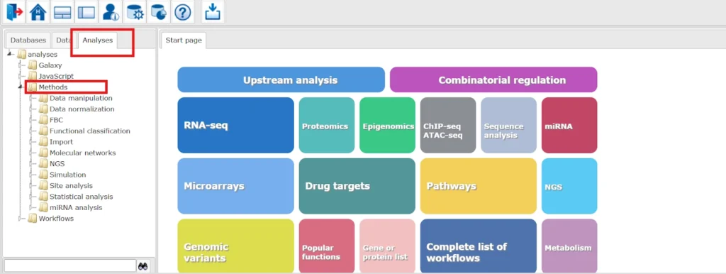
All analysis methods can be found under the Analyses → Methods folder. These methods are organized according to the type of analysis you want to perform.
Most methods are straightforward and can be executed with just one click:
- Open the desired method in the workspace.
- Select the input (e.g., a gene table from your folder) in the input form.
- Specify the output path and choose an output name.
- Press Run to execute the method.
Here we will summarize, some most common methods for a better understanding of the geneXplain platform
- Gene set to track
The Gene set to track method allows you to create a genomic track from any table containing Ensembl gene IDs. This track is built around the transcription start sites (TSS) of the selected genes, and is especially useful for generating promoter or upstream region tracks.
By default, regions include 1000 bp upstream and 100 bp downstream of each TSS. The resulting track opens in the genome browser and shows fragments with chromosome, position, length, strand, and type information. All additional columns from the original gene table are preserved in the new track.
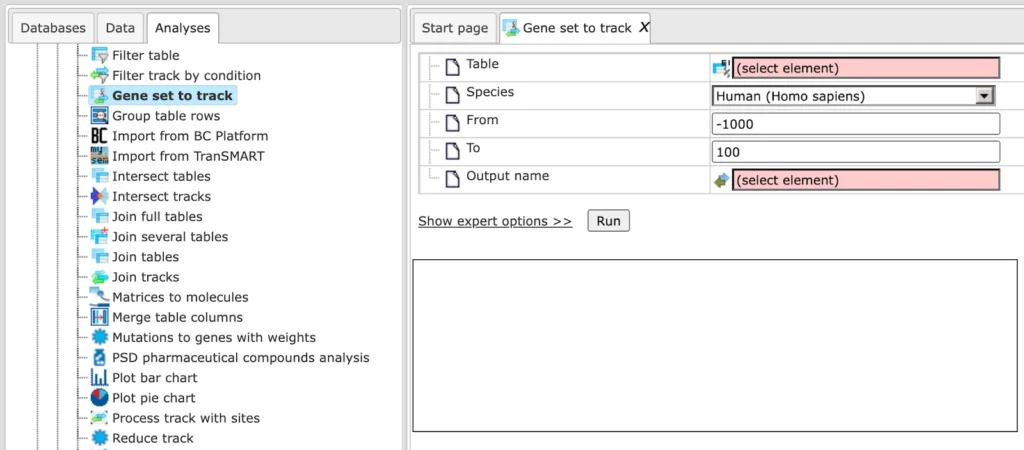
Input table: Specify the input table with Ensembl gene IDs. If your table has different IDs, you need to convert it first. You can drag & drop the table from your project within the tree area. Alternatively, you may click on the pink field select element and a new window will be opened, where you can select the table.
Here we are using the sample Ensembl gene list
Species: Once the table is loaded, the species (human, mouse, or rat) is detected automatically. Confirm that the correct species is shown.
Region (From/To): By default, the method selects 1000 bp upstream and 100 bp downstream of each TSS.
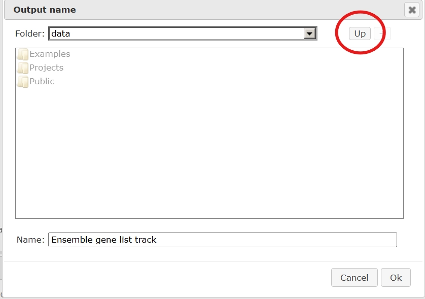
Output name: Specify the output track name and location, you can select the location using the arrow keys as shown below, and save the output track in your projects
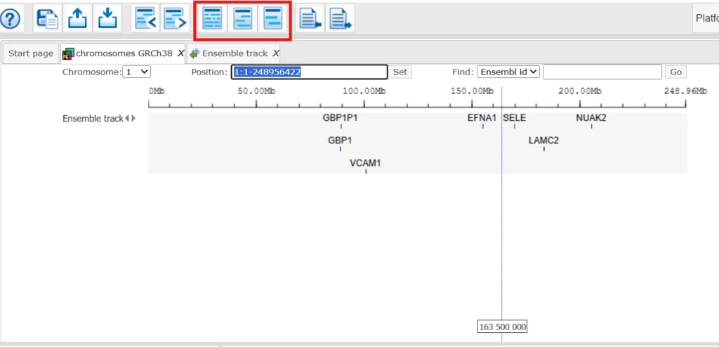
click Run. When the analysis is complete, the resulting track opens automatically in the genome browser of your workspace.
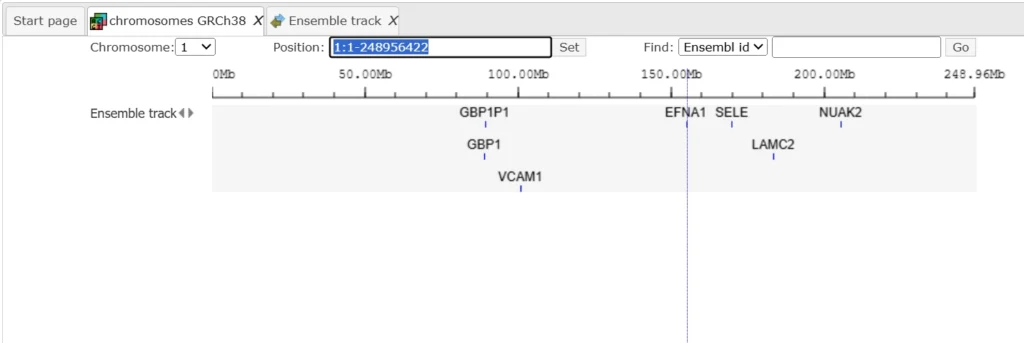
You can use these buttons to visualize the track in detail.
Right click on the track and you can open the track as a table. This table contains exactly the same number of the fragments (rows) as the number of Ensembl genes in the input table. There are columns for chromosomes, positions From and To, Length, Strand, and Type. The type of the fragments after this conversion is automatically assigned as misc_feature. Other columns present in the input table are all added on the right side of this table, e.g. here Affymetrix ID column.
For the following methods, please, refer to the respective tutorial videos :
In addition to gene tables, the platform provides full support for track files, BED files, and interval files (represented by the symbol (![]() )).
)).
A variety of processing methods are available, including conversion of tracks into tables, filtering, and joining tracks. All methods are designed with a straightforward click-and-run workflow: users simply supply the required input data and execute the method.
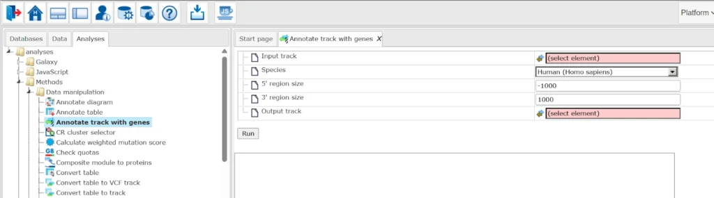
Annotate track with genes
The Annotate track with genes method links each fragment in a track to nearby genes. It compares fragment positions with extended gene regions (by default: 1000 bp upstream of the TSS and 100 bp downstream of the last exon) and adds information about any overlapping genes.
Simply select your input track, confirm the species (human, mouse, or rat), adjust the upstream/downstream ranges if needed, and run the method. The annotated track opens automatically in the genome browser and contains the original fragments along with gene annotations.
You can use the track of your choice or can use the sample track.
Once we run the sample track the output track is opened automatically, when opened as a table it looks as shown below:
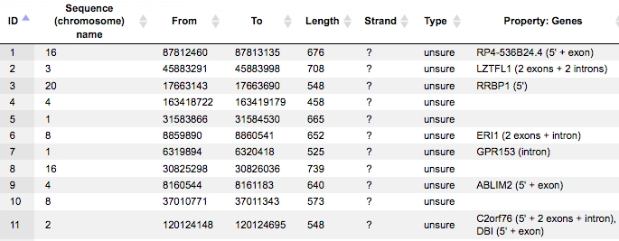
All columns of the input track are present, and one column is added, called Property:Genes.
This newly added column is a result of an annotation of the input track with genes, and for each fragment it contains gene symbols of overlapping genes. As you can see, some of the fragments are not overlapping with any genes, and some of the fragments may be overlapping with two or even more genes. It depends on the particular fragments, their length and location as well as on the length of the gene-bound extension regions specified in the input form.
Next to each gene symbol there are gene regions specified, for example ERI1 (2 exons + intron). This means, a particular fragment overlaps two exons and one intron of the ERI1 gene.
Tip: If you would like to annotate overlapping genes for all fragments in the input track, you might be interested to increase the gene-bound extension regions in the input form, and run the analysis again.
Process track with sites
In general, a track is a set of intervals where positions are specified that we can map on a chromosome. These track files can be visualized in a genome browser and can be used as input for various site analysis functions.
The geneXplain platform provides you with an option to modify these track files. “Process track with Sites” is a function which enables the user to enlarge/shrink sites on the track, merge overlapping sites or remove too short sites. For example an already saved track in the repository can be processed by adding sequences from Ensembl or some other database.
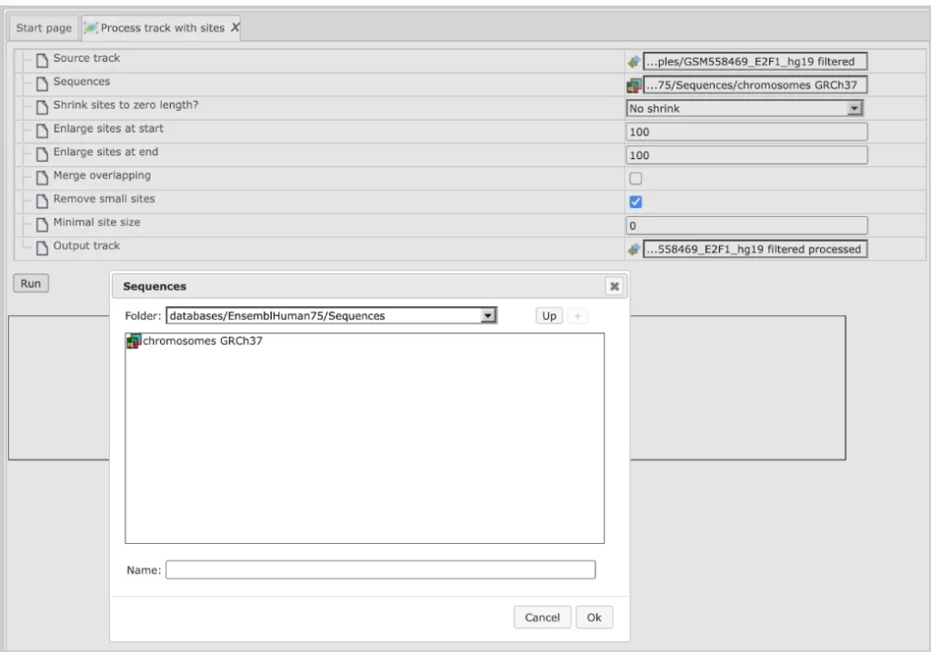
The initial form of this analysis looks as shown below:

Source track: Track you want to process
Sequences: Sequences to use
Enlarge sites at start: Use positive numbers to enlarge and negative to shrink
Enlarge sites at end: Use positive numbers to enlarge and negative to shrink
Merge overlapping: Checking this box merges overlapping sites into a single site. Site annotations will be lost!
Remove small sites: If checked, sites smaller than Minimal site size will be removed, otherwise they will be expanded to Minimal site size
Minimal site size: Sites shorter than the specified size will be removed from output
Output track: You should specify the path for the processed track here.
The track file shown provides you with the positions of promoter areas selected for analysis, as shown in columns From and To. The column Strand shows the strand of the chromosome where these promoters are located, where 1 means strand not applicable, 2 means forward strand, 3 means reverse strand, 4 means both strands. This file can be dragged and dropped on a particular chromosome opened in the genome browser to visualize its positions.
This Source track file can be selected as an input to “Process track with Sites”. The sequences we want to map are selected from the Ensembl database as shown below:
Using default conditions for the other parameters you can now press [Run].
Sample input and Output files can be checked in the platform.
These processed track files can be used for other site analysis workflows.
Venn Diagrams
With this feature you can create VENN diagrams from the input tables as well as to get tables of common and unique genes according to the sections of the VENN diagrams. VENN diagrams are images that show all possible logical relations between the input tables.
As input, two or three gene tables can be provided for which you wish to know common and unique genes. These input tables can be in any format (gene or protein IDs). The VENN diagram function can be found under the tab Analyses, in the folder Methods/Data manipulation/Venn diagrams.
The initial form of this analysis looks as it is shown below:
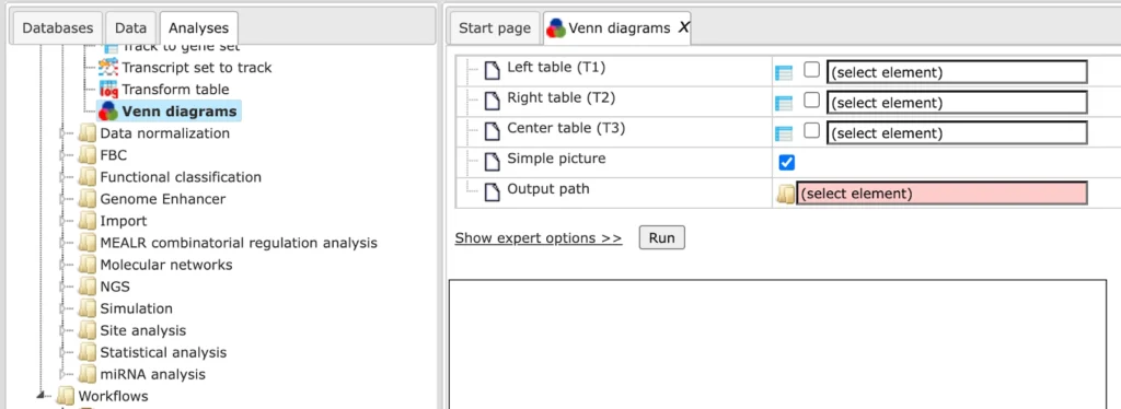
Under the expert options you can see more options to change the color of the diagram. Left-top circle color, Right-top circle color, and Center-bottom circle color. In these fields you can specify the colors you wish to see in the diagram.
Simple picture. When this box is checked-, all three circles in the resulting diagram will have the same size, no matter whether the input tables are of the same size or not. By default this option is checked.
When this box is unchecked, the size of the circles will be proportional to the size of the input tables in the resulting diagram.
Input 2 or 3 gene list for which you want to create the Venn Diagram, specify the output path and press ‘Run’.
Check the sample Input files and Output files in the geneXplain platform public folder.
Identification of differentially expressed genes using Guided linear model analysis
You can identify differentially expressed genes for a gene list using the method Guided linear model analysis
This method can be found in the methods section/ Statistics folder
This tool performs a linear model analysis on the input table, guided by experimental factors defined in a sample table. It identifies significant differences between pairs of levels within the main factor and conducts an ANOVA across all contrasts. The assignment of main factor levels to input columns is specified in a sample table column. Additional variables can be controlled by listing their column names, and Surrogate Variable Analysis (SVA) can be included to detect hidden factors.
Ensure that input table column names match the row names of the sample table. If different identifiers are used, specify the correct column using the Sample column parameter. To analyze only specific columns, define them in the Data columns parameter.
Avoid using numerical names, and make sure all column/sample names follow R naming conventions.
Confirm that Input type and Normalization method are correct:
- Raw counts → processed with Limma’s voom, optionally normalized.
- Normalized values → used directly.
- Transformed counts → analyzed with eBayes (trend = TRUE) to include intensity-based trends.
Input form looks like:
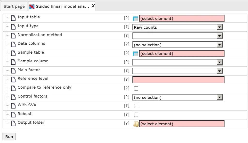
Input parameters:
Input table – Path to the file containing your input data.
Input type – Type of data provided (e.g., raw counts, normalized, transformed).
Normalization method – Normalization method to use with voom.
Data columns – Optionally choose specific columns from the input data.
Sample table – File containing sample (column) information.
Sample column – Column in the sample table that lists sample names (used if row names are not samples).
Main factor – The main experimental factor to compare.
Reference level – Optional base level; other levels are compared against this one.
Compare to reference only – Limits analysis to comparisons between the reference and other levels.
Control factors – Optional additional factors to control for (columns from the sample table).
With SVA – Enable Surrogate Variable Analysis to account for hidden variables.
Robust – Use a version of the analysis resistant to outliers.
Output folder – Folder where all results will be saved.
Sample Input file used:
Sample meta-data
Output:
The list of differentially expressed genes can be filtered as per requirement and used further for different workflows.